The model is used to derive analytical expressions for the relative income returns to entrepreneurship which are defined in two ways: in relation to the income from observationally similar wage in employment and in relation to the counterfactual income of entrepreneurs as wage in employment. The model-based income distributions for entrepreneurs and wages in employment match the observed distributions. Earlier empirical studies of the income differences between entrepreneurs and wage workers and our own income distribution data provide some hints for the specification.
Comparing our two measures of the relative income return to entrepreneurship, we also show that the self-selection bias inherent in empirical income return studies that compare observationally similar entrepreneurs and wage earners is likely to be larger the higher the observed relative frequency. If s1, both entrepreneurs and wage earners will earn more on average than they would by making the opposite occupational choice. With the same distributional assumptions, we can also derive closed expressions for the expected incomes of entrepreneurs and wage earners.
From proposition 4 this is fully consistent with the fact that entrepreneurs on average earn less than the similarly employed observer wage. Considering the modified Lazear model with the same assumptions as in Proposition 2, Proposition 5 in Appendix A5 provides closed-form expressions for the relative expected income returns to entrepreneurs and employed wages E and W, respectively.

The data
We will make a distinction between all self-employed and the subgroup of self-employed who hire at least one person, the latter being denoted 1+. Furthermore, we will consider individuals who are employed or self-employed in 2008, as well as those who enter the labor market in 2008 and become either self-employed or wage-employed. The corresponding percentages of self-employed employing at least one individual are about half as high among electrical engineers and architects, but significantly lower for non-performing artists.12 A possible explanation could be that it is easier to find a job or at least to get a job. corresponding to the education, for electrical engineers.13.
As can be expected, the share of self-employed persons who employ at least one individual is lower among entrants than among all employees. 12 The upper part of each panel compares all self-employed with all employees, and the lower part compares the subset of self-employed who employ at least one person with all wages. 13 As shown in Table B1, the average income for employed electrical engineers is considerably higher than for salaried architects and non-performing artists.
Percent returns of the self-employed and relative earnings defined as median earnings of the self-employed as a percentage of median wage earnings of the employed in 2008 by education. The top half of each panel includes all the self-employed and the bottom half only the subset of the self-employed who employ at least one person (1+). But an electrical engineer who belongs to the category that also includes all self-employed will earn an average of 49.5 percent less.
Our model provides some information about possible reasons for the differences in income returns between all self-employed and self-employed who employ at least one person. Y according to Theorem 4, and s is the adjustment factor for utilities, could be an explanation that self-employed people who hire others value disadvantages caused by risks, for example, and positive benefits, such as self-employment, are less important. more important than the self-employed on their own account. The 5th income percentile is, with one exception, lower for the self-employed than for wage earners.
The pattern is somewhat less clear at the upper end of the income distribution, but the 99th income percentiles indicate that all self-employed tend to be overrepresented, assuming they employ someone, and that entrants are overrepresented throughout.
Results
As shown by the top of Panel A, the returns to self-employment are -2 percent for electrical engineers, 30 percent for architects, and 3 percent for non-performing artists. The returns to self-employment among those who employ others are positive throughout and also higher than among all self-employed for both Panel A and B.15 Income returns to wages. Apparently it seems to pay much better – on average – to start a firm and hire others than to become gainfully employed for newbies in the labor market. 16.
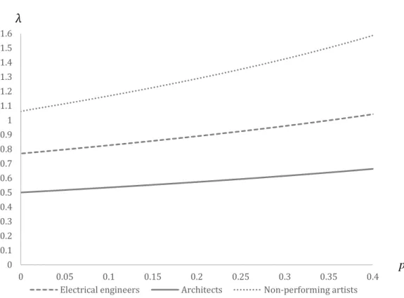
As we explain in Section 2, self-employment income return measures of the kind presented in Table 1 are biased by self-selection and this bias will increase with the observed relative frequency of self-employment. A possible explanation is that the trade-off between the dangers of entrepreneurship and the security of wage employment is more important than the possible benefits of being one's own boss for various categories of the self-employed. Using the parameter values for all incoming electrical engineers, architects, and non-performing artists, Figure 2 illustrates the corresponding supply curves.
16However, the high returns are quite uncertain due to the small number of self-employed persons who employ others, see table B1 in Appendix B. The S and values are chosen in accordance with table 2, panel B: all self-employed -employed versus wage-employed. As shown in Proposition 3 in Appendix A3, the income distributions for wage earners and entrepreneurs can be derived if the strength of their skills is assumed to be Fréchet-.
It is somewhat better for employees than for the self-employed and about the same for all self-employed people as for self-employed people who employ others. For participants, i.e. panel B, the calculated percentiles deviate more from the observed ones, especially among electrical engineers and non-performing artists. It should again be noted that there are only a small number of self-employed participants in panel B, and their observed income distributions are therefore particularly uncertain.
An obvious improvement would be to control for observable individual characteristics such as age, gender and labor market region and to use after-tax instead of before-tax incomes.18 Another possibility is to use time series information and, for example, consider the choice of wage employed to remain as wage employed or to become self-employed, and to include previous experiences with wages and self-employment as additional characteristics.

Concluding remarks
The ratio between calculated and observed income percentiles in the year 2008 according to education and occupational status. The calibrated values of the utility adjustment factor indicate that risk consideration may be as important as non-monetary benefits for the choice between self-employment and wage employment. The main contributions of the paper are the derived upper and lower bounds for the relative income returns to entrepreneurship defined in counterfactual terms, the statement that lower expected earnings for entrepreneurs than for wage employment is fully compatible with the Lazear model, and the derived measure of the self-selection bias inherent in estimates of the relative income returns to entrepreneurship defined in terms of observationally similar wages employed.
More generally, the paper emphasizes the importance of considering both the positive and the negative non-economic aspects of entrepreneurship as well as making explicit assumptions about the distribution of skill profiles. If the occupational choice is based solely on income maximization (p1), then all entrepreneurs will earn more than they would if they had been forced to make the opposite occupational choice for some reason. But whether utility maximization will result in higher or lower expected earnings for entrepreneurs than for wage earners depends on the assumptions made about non-economic benefits and. distribution of skill profiles in the population.
It follows that alternative assumptions about the utility adjustment and the skill distribution can also solve the so-called income puzzle with entrepreneurship. As an alternative to the Fréchet distribution, the Weibull distribution, that is, another extreme value distribution defined for positive values, is an obvious candidate to test. An extension will be to investigate the possibility of estimating the market value of entrepreneurial talent as a function of individual characteristics such as age, gender and their labor market region.
Since the income returned to entrepreneurship and wage labor should ensure that the supply of entrepreneurs and specialists matches the demand, a more ambitious theoretical extension would be to develop a labor market model that allows simultaneous measurement of the market value of entrepreneurial talent and the parameters of the skill profile distribution.19. The empirical tests of Lazear's model (reported by Aldén et al. 2010) can be supplemented with estimates of the parameters of the Fréchet distribution, or other distributions of skills profiles, and the resulting implications for self-employment rates and earnings.
Appendix A. Additional propositions, proofs and parameter calibration
We want to show that b as a function of pE strictly decreases on the interval (0,1).22 It is somewhat simpler to prove the equivalent statement that b as a function of pW 1 pE strictly increases on the interval (0,1). To apply the modified Lazear model as specified in Proposition 2, four parameters must be calibrated against empirical data: , ,s and v . We will use pE as our observation for pE, and YE and YW as our observations for E[ YE] and E[YW], respectively.
Finally, s is determined so that the sum of the squared deviations between the p-percentiles of the observed and calculated income distributions of entrepreneurs and wages in employment is minimized: 23. The averages of the observed and calculated incomes will be equal and the sum of squared differences between observed and calculated income percentiles are minimized.
Appendix B. Additional data
Panel B: All participants who become wage employees, self-employed and the subset of self-employed who hire at least one person (1+). Perceived income percentiles in the year 2008 by education and occupational status (in thousand SEK per year).

Acknowledgement