ELECTRIC FIELD

These zero-field states are used to expand the eigenstates of the helium atom in the non-zero external electric field. Furthermore, the decrease in the intensity of the (n−1)c/nb 1Po doublet is attributed to the coupling of optically allowed 1Po states to strongly autoionizing 1Se (forF kP) and 1De resonances (forF kP and F ⊥P), whereas the broad peaks following the na 1Po resonances are shown with high steps in the N value to the 2 origin threshold state near the N value . a.

Overview

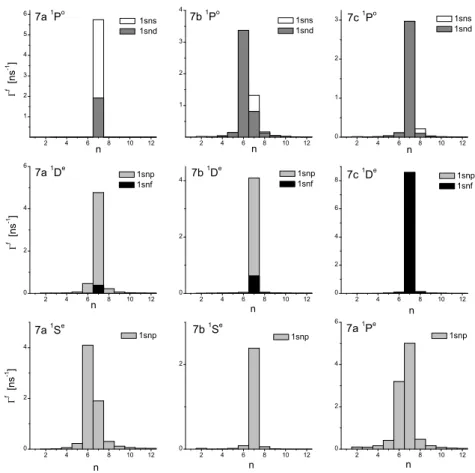
Calculations show that the fluorescence of all doubly excited states below N = 2 exhibits lifetimes of the order of 100 ps. The lifetime of the first member of the series (n= 3) was measured with a beam-sheet technique [30] and determined to be 110±20 ps, again in agreement with the theoretical description [20].

Figure 1.1: Schematic energy diagram of helium. In this work we study the photoexcitation of resonances below N = 2 threshold in the static electric field and their decay by the autoionisation (dotted line) and fluorescence.

Motivation and outlook

However, none of the six even series can be observed in simple photoabsorption due to the selection rule that requires a parity change. Above H0 and ∆H denote the free atom Hamiltonian and the interaction of the atom with the electric field.

Correlation quantum numbers

T describes the magnitude of the l1·ˆr2 overlap, or roughly, the relative orientation between the two electron orbitals. Members of the same series are numbered by quantum number n, starting from the lowest value available (this can be checked by considering different configurations of the given LSπ symmetry where the (inner) electron is confined ton1=N).

The Stark effect

Splitting the Schrödinger equation into parabolic coordinates is still effective in the non-zero field. It was shown to appear naturally in the two-center adiabatic approach [63], as the eigenvalue of the body-fixed electron exchange operator, which can only assume values ±1.

Figure 2.1: The Coulomb potential of the nucleus is modified by the external static electric field, allowing an electron to tunnel through the barrier.

Propensity rules

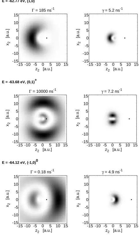
The maps of the conditional reduced probability density computed from the correlated states 1Po with n=3 clearly show the Stark character following from the state notation (Fig. 2.3) [56]. To end up with A=−1 states, one of the electrons, after photoabsorption, has to change its direction of rotation, and this is much more difficult than just changing the orientation of the orbit.

Experimental

At the beginning, we explore the simplest possible approach for quantifying the fluorescence yield from doubly excited states in an electric field – first-order perturbation. A first-order even singlet state with a projection M of the angular quantity Lis given by.

Results

For a reliable description of the individual and doubly excited states of the helium atom in the homogeneous electric field, accurate wave functions of the atomic eigenstates are needed. The usual variational approach involves optimizing the nonlinear parameters of the basis functions before diagonalization.

Figure 3.2: Comparison of the experimental VUV photon yield and calculated primary fluores- fluores-cence yields from the 1 P o state (green line) and 1 P e , 1 D e states (red and blue line) perturbed by the electric field of 5 kV/cm (F ⊥ P ).

Hamilton operator in Sturmian basis

This can drastically reduce the size of the relevant matrices and therefore allows higher angular momenta to be included in the calculation. As already mentioned, more details on the numerical treatment of the problem will be given in Chapter 5.

The method of complex scaling

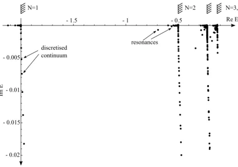
For Θ>0, the discrete part of the spectrum H(Θ) is associated with a wave function that behaves asymptotically as an outgoing wave if the imaginary part of the eigenvalue is different from zero [87, 88]. In general, it holds for the eigenstates of the complex scaled Hamiltonian for the generalized complex scaling inner product [88].

Figure 4.1: Left: the spectrum of the unrotated Hamiltonian. Black circles denote bound states.

Interaction of an atom with a radiation field

To find eigenvalues EpΘ and eigenvectors |ΦpΘi of the total complex, the Hamiltonian H(Θ), is scaled. an extension analogous to Eq. A(r) is the vector potential of the radiation field. 4.49) runs over two linearly independent polarizations (denoted by the index β) and over all possible values of k in the normalization volume V.

Photoionisation cross section

Fano profile
Fano profile with radiation damping
Field free photoionisation
Spontaneous emission
Photoionisation in electric field
Spontaneous emission in electric field

According to the latter, the integrated cross section is equal to the squared modulus of the dipole matrix element between the undisturbed bound state (denoted by |ϕi) and the initial state. The contribution of the continuum term can be treated in the same way as the photoionization cross section [cf. Similar treatment to the no-field case applies to the outer-field case.

Figure 4.4: (a) Fano profile [Eq. (4.64)] for different values of parameter q. The profiles for negative values of q are obtained by replacing ǫ with − ǫ

Inelastic photon scattering cross section

Field free scattering

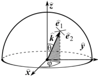
The completeness relation of scaled complex eigenstates is used and the initial and final state are expressed in terms of their complex scaled counterparts. Since the eigenvalues are independent of the magnetic quantum numbers, the angular integration can be performed by means of the parametrization of ˆk and ˆeβ described in Appendix B. Their asymmetry is a consequence of the interference with continuous and nearby resonances and associated states (the total energy width of the last dekaiteity may be radiative due to the latter).

Inelastic scattering in electric field

A pseudo inverse of the overlap matrix is possible, however, if singular value decomposition (SVD) is used to determine the linearly independent vectors [104]. Smaller eigenvalues, however, that are close to the numerical errors of the matrix elements are less accurate than in the SVD case. 5.8), the matrix B can be approximated by P selected eigenvectors and eigenvalues σj,. 5.13) is a common eigenvalue problem for the column vector x′i =S′−1xi, where.

Eigenstates and eigenvalues of the total Hamiltonian

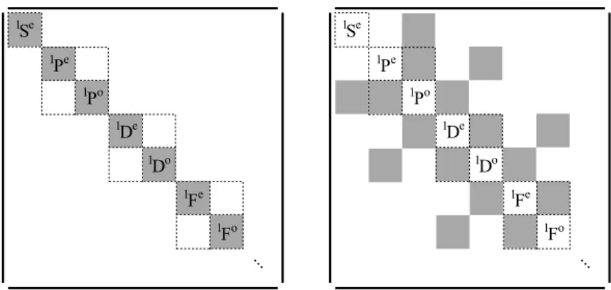
Let the submatrices of H0(1Lπ) and S′(1Lπ) have the following dimensions, consistent with the notation used in the previous section:. 5.20) With the latter forms of H0 and S′, the Hamiltonian operator is written in reduced representation as. The meaning of Bij is the following: ifx′i represents an eigenstate of symmetry 1Lπ11 and x′j an eigenstate of symmetry 1Lπ22, the matrix element. In practice, the eigenproblem for each of the symmetries 1Lπ is calculated and diagonalized separately to save space.

Construction of the basis set

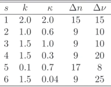
According to the independent electronic model for a chosen L, there are three Rydberg series for doubly excited states with parity π = (−1)L under N = 2. The parameters from Tables 5.1 and 5.2, improved by Sturm functions with ks and κs replaced, are used to obtain the energies of singly and doubly excited states from Appendix E. Finally, it should be said that although the basic parameters are optimized for states below N = 2, calculations show that with the basic i arrays such as the one presented in Tables 5.1 and 5.2, doubly excited states approaching higher thresholds, specifically N = 3 and N = 4, are also obtained in the same diagonalization.

Table 5.1: Nonlinear scaling parameters k and κ used in the calculation of 1 D e basis states.

Implementation

Radial integrals

Results are reported to nine decimal places, but calculations are not checked for accuracy. Since the integrals involving the operators of individual particles of the entire Hamiltonian have the form (cf. Appendix B). In order to be able to use the quadrature formula (5.30) to evaluate the integrals in Eq. 5.33), the order of integration in the first term on the right side changes and the substitution r1 =r2(ξ+.

Calculation and diagonalisation of the Hamilton matrix

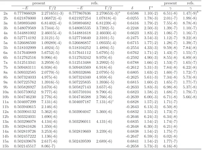
Because the matrix sizes of the individual matrices involved in the calculation are relatively small, an exact diagonalization is used. The computer codes for the calculation of matrix elements of the matrices H0(1Lπ) and H, photoionization and inelastic scattering cross-section, and various utilities are written in C++. Most of the existing values for doubly excited states refer to 1Se (up to n = 15) and to 1Po series (up to n = 10) while for the few other series (1Pe, 1De, 1Do, 1Fo and 1Ge) only the numbers for the lowest lying members have been previously published.

Stark maps

We have accurately calculated singly and doubly excited singlet states up to ton= 15 and up to the total angular momentum L≤10 in the zero electric field. We could not find any previously published data on doubly excited states with 1Fe and 1He,o−1Ne,o symmetry. As mentioned before, these states were further used to represent doubly excited states in the non-zero electric field.

Photoionisation

Comparison with experiment

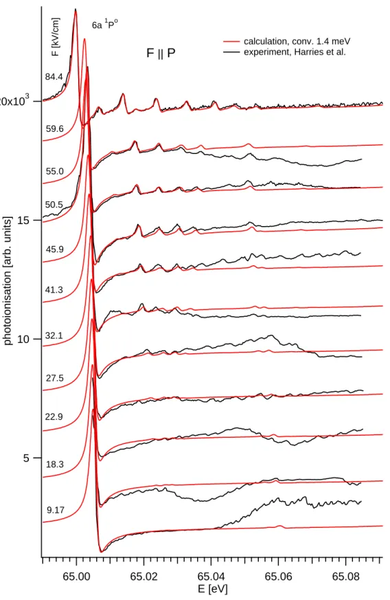
The energy scale of the calculated spectra is used for alignment of the measured photoionization signal. The experimental data is scaled to match the amplitudes of the calculated peaks, and the spectra are retranslated along the ordinate. A complete set of calculated spectra for all values of electric field strength and both polarizations is shown.

Identification of states and the propensity rule

With the basic Stark map, the identification of peaks in photoionization spectra is greatly simplified. The Stark maps of the energy region n = 6 and = 7 using the scheme a∗b∗c∗ are shown in Fig. The left plot shows the LSπ symmetry of the principal components of the states (cf.

Figure 6.4: Comparison of measured and calculated photoionisation cross section for various field strengths for F k P

Inelastic photon scattering cross section

Comparison with experiment

Analysis of the fluorescence yield spectra

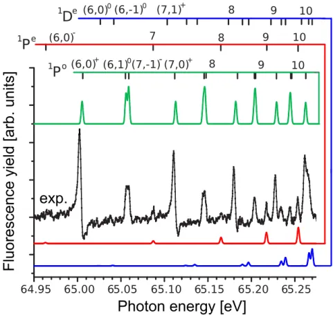
The calculated spectra are scaled and Gaussian-broadened with 3 meV FWHM (2.5 meV FWHM for 0 kV/cm) to match experiment. The blue curve represents the photon scattering signal, the green the ion signal, and the red curve their sum.

Figure 6.14: Comparison of the spectra measured by Prince et al. [47] and the calculated total fluorescence yield for F ⊥ P

The time domain

We devised the procedure to obtain the inelastic photon scattering cross sections using the eigenstates of the Stark Hamilton operator in complex space. The direct observations of the total decay rate of resonances are possible in the time domain. In this appendix, the expressions for matrix elements of the Hamiltonian operator in the basis of Coulomb Sturmian functions are derived.

Figure 6.20: The measured (top) and calculated (bottom) photoabsorption and photoionisation cross sections

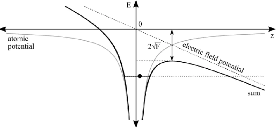
Potential energy

The last equality derives from the known orthogonality relations of spherical harmonics and spin functions. The expression can be simplified, since the radial integrals are symmetric with respect to the exchange r1 ↔r2,. Appendix B - Matrix elements of the Hamiltonian operator in the Sturm basis 115 The radial integrals in Eq.

Electron-electron interaction

Overlap matrix elements

Spherical dipole operator

Using this last property, Eq. Appendix B - Matrix elements of the Hamilton operator in Sturmian basis 117 with. B.29). The Wigner-Eckart theorem can now be used to calculate the total matrix element: . hψknlκνλLS.

Electric field interaction

Dipole transition operator

Reduced dipole matrix element of complex dilatated states

Dipole matrix elements in electric field

In the following, the formulas for the convolution of the calculated theoretical spectra with the Gaussian are derived. In this appendix, the parameters of the singly and doubly excited singlet states of the free helium atom used in the calculations are tabulated. The method is combined with complex scaling to calculate the energies and autoionization widths of a set of doubly excited states of 1Se.

Figure C.1: Photon emission in the direction ˆ k: ˆ e 1 and ˆ e 2 are two mutually orthogonal polari- polari-sation vectors.

Doubly excited states

Skoraj do poznih devetdesetih let prejšnjega stoletja je avtoionizacija veljala za prevladujoč kanal razpada dvojno vzbujenih stanj z vrtilno količino L = 1. Učinke zunanjega polja na primarno in sekundarno fluorescenco dvojno vzbujenih stanj pod drugim ionizacijskim pragom so opazovali v domeni časa in energije. Zato predstavljamo prve celovite izračune ionskega izkoristka v območju dvojno vzbujenih stanj helija v močnem električnem polju.

Table E.12: Doubly excited 1 S e states.

Formulacija problema

Obravnava problema

Z Greenovim operatorjem in lastnimi stanji Hamiltonovega operatorjaH(Θ) lahko enostavno izrazimo fotoionizacijski presek, ˇce obravnavamo osnovno stanje kot vezano (gl. npr. Chapter F – Razˇsirjeni povzetek v slovenˇsˇcini 149 V enaˇcbi (F.8) smo upoˇstevali le prehode v konˇcna enojno vzbujena stanja |ΦiΘi, ki jih obravnavamo kot vezana tudi v prisotnosti polja. Integracija v enaˇcbi (F.8) poteka po smereh valovnega vektorja izsevane svetlobe k, z ˆeβ,β = 1,2, pa smo oznaˇcili linearno neodvisni polarizaciji izsevanih fotonov.

Rezultati

Starkovi diagrami

Predpostavili smo, da je osnovno stanje vezano, za vezana pa štejemo tudi končna stanja |ΦmΘi, zato smo postavili Em = ReEmΘ. Vsota do m vključuje le nekaj vzbujenih stanj v električnem polju, medtem ko vsota do n zajema vsa stanja, ki so dosegljiva z absorpcijo fotona iz osnovnega stanja.

Fotoionizacija

Kot je razvidno s slik, potrdi raˇcun ve- ljavnost pravila tudi za pravokotno eksperimentalno postavitev (F ⊥P), kjer ostajajo amplitude vrhov z vodilnimi komponentami tipa b∗ inc∗ razmeroma majhne tudi za stanja zn= 7.

Neelastiˇcno sipanje fotonov