Before starting to use the routine, you should load the file init.m from the root folder of the routine. This file adds the necessary directory paths to Matlab's PATH variable and also loads the set of method parameters with their default values. To start using the routine, one might want to define their own map to study.
For this it is enough to create a new Matlab script file with the appropriate function, the typical view of which is shown in Listing 1 (see also Listing 2, other default sample files in the routine/ directory map, and the package documentation Matlab [1] for more details). A Jacobi matrix for the user-defined map can also be provided explicitly, which appears to be useful when finding periodic points (by Newton's method) and computing their eigenvalues and eigenvectors. First, it gets the data for the diagram and then uses this data to make the 2D color chart.
The method of obtaining period data is quite straightforward: starting from the given starting point, a target map is repeated the specified number of times, and then the last point reached is checked to be periodic (where the period is not greater than the given maximum value).
Obtaining period data
This is because for any pair of parameters, the initial value is always reset to x0 if it is a numeric array. However, one can force the initial condition to be chosen randomly at each cycle change by specifying x0 as a string of the form 'rand(
It should be mentioned that for the two target parameters (which will then be varied to obtain the diagram), one must give their values here as well, although these values will not be used. Note that the value -1 corresponds to the orbits diverging to infinity, and 0 is related to either the case of non-regular (eg chaotic or strange) behavior, or to the orbits of period greater than maximum period. The return values from period_bd_calc can be used directly in bd_plot for plotting the bifurcation diagram.
While running, the function displays information about the data calculation progress in the command window. At each cycle turn, when the first parameter changes, its current value is displayed in orange, and the approximate time remaining is displayed in blue.
Plotting period diagram
It is limited to a maximum of 62 colors, where gray corresponds to -1 (divergence) and white corresponds to 0 (higher periodicity or irregular behavior). Note that if matrix C contains cells with values greater than the maximum period, these will also be colored white on the generated graph. To find periodic points, the Newton-Raphson method is used to approximate the zero roots of a function (see e.g.
The method for 1D maps is implemented in the function find_periodic_1d (see file main/find_periodic_1d.m). Note that it is also possible to find points with periods that are divisors of the period. If false (or 0), the search interval is divided into init_num equal parts, and then the midpoint of each subinterval is taken as the initial condition.
While running, the function displays information about the calculation progress in the command window. Each run (initial condition tried) number appears unorange, the total number of Newton steps is displayed in blue, and if the Newton method does not converge, a warning is displayed in green.
Multi-dimensional maps
They can be given either as a simple comma-separated list, or as a single cell array parameter (see Listing 11 and example/do_points_sample.m, note that {:} is important).
Classifying found periodic points
Fixed points
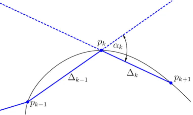
To calculate the unstable manifold of a fixed point one must use the function sc_unstable defined in main/sc_unstable.m. Note that if d > 0 manifold is grown forward, while if d < 0 it is grown backward. If the angle α between the vectors (pk−1, pk) and (pk, pk+1) falls below this value, the step size is increased.
It is assumed that the angle α between the vectors (pk−1, pk) and (pk, pk+1) does not exceed this threshold (for exceptions, see [4]). Da_min Minimum value for the product ∆kα, where ∆k is the current step size and α is the angle between (pk−1, pk) and (pk, pk+1). Da_max Maximum value for the product ∆kα, where ∆k is the current step size and α is the angle between (pk−1, pk) and (pk, pk+1).
If the distance between the point ˆpk+1 (where ˆpk+1 is a candidate for the next division point pk+1) and the said circle is less than cB ·R, where R is the current circle radius, the point pk+1 is assumed found and the division stops. To better understand the role of the parameters a_min, a_max, Da_min, Da_max, D_min and cB, it is recommended to refer to [4] and other works by the same authors. Information about the progress of the calculation is printed in blue, warnings (e.g. about inability to find the next point, or accepting the point that does not meet the required constraints - for details see [4]) appear in the green.
Certain auxiliary information is displayed in orange, and the final data is printed in violet.
Periodic points
The angle α between the vectors (pk−1, pk) and (pk, pk+1) is assumed not to exceed this threshold (for exceptions see [4]).
Stable manifolds
Fixed points
To calculate a stable fixed point manifold, the sc_stable function defined in main/sc_stable.m must be used. This parameter is useful in the case of a non-invertible map that may have multiple preimages. The stable manifold of such a map can be mapped onto itself in a complex way, so that it is necessary to repeat the map several times until we get the right approximation for the next point (see [5, example 4.3]).
Note that if d > 0 manifold is grown forward, while if d < 0 it is grown backward. To understand more deeply the role of the parameters a_min, a_max, Da_min, Da_max, D_min and eB, one is encouraged to refer to [5] and other works by the same authors.
Periodic points
Plotting computed manifolds
Lambda_noinv.m is a particular non-reversible card logistic_J.m derivative of the logistic card logistic.m logistic card. The method used to construct invariant manifolds is the Search Circle Algorithm (SCA) [4, 5], which grows one-dimensional manifolds in steps by adding new points according to the local curvature properties of the manifold. The difference between the SC algorithm and other methods is that it does not require the reverse.
It finds a new point close to the last computed point that is mapped under the function f to a part of the manifold that was already computed.
Growing the manifold
The manifold is forward invariant, so new points, and in particular pk+1, must be mapped to the part of the manifold that has been computed so far. Thus, we are trying to find a point pk+1 at a distance ∆k from pk such that f(pk+1) belongs to a segment of the already calculated part of the manifold1. For this we draw a circle C(pk,∆k) of radius ∆k with a center at pk (green color in Fig. 1).
The image f(C(pk,∆k)) is then a closed curve (magenta color in figure 1), which is located near a certain segment of the already calculated manifold. For this the method proposed in [6] is used, namely assuming that the angle αk between the lines drawn by pk−1, pk and pk, pk+1 (see Figure 2) is within certain limits. 1Note that in certain cases of non-invertible mappings the point pk is mapped not by f, but by an iteration fm of the previously computed part of the manifold.
We can immediately ensure that αk does not exceed αmax by searching only the part of the circle C(pk,∆k) that meets this criterion. To control the local interpolation error, we also check that the product ∆kαk lies between (∆α)min and (∆α)max. This ensures that the number of points used to approximate the manifold is in some sense optimized for the required accuracy constraints.
Finally, to find pk+1, we need to define which segment of the previously calculated manifold contains the intersection with f(C(pk,∆k)). To find the candidate for pk+1, we use the bisection method for the angle αk, and let the point f(pk+1) be at a maximum distance of a small εB (the bisection error) from the detected segment, for example , Ij = (pj, pj+1), of the previously calculated manifold part. Note that in this procedure the points f(pstart) and f(pend) must lie on opposite sides of the segment Ij.
If not (for example, if there is a sharp crease in the manifold), the search area for angle αk is enlarged and a warning message is printed. We take the image of the arc between pstart and pend and check that iff(pstart) and f(pend) lie on either side of the line through pi−1 and pi. Finally, if the angular search area is enlarged and αk > αmax, we also check whether ∆k < ∆min.

Unstable manifold