This is a new, deformation theory-based treatment of the parametrization developed here with a complete treatment of infinitesimal deformations and constraints for several related functions. In fact, this part of the book is intended for a more advanced reader familiar with the basics of modern algebraic geometry and commutative algebra.
Singularity Theory
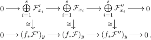
We show, as an application of the finite coherence theorem, that they behave semicontinuously under deformation. One of the most important geometric characterizations of plane curve singularities is based on the embedded resolution (desingularization) via subsequent blow-ups.
1 Basic Properties of Complex Spaces and Germs
Weierstraß Preparation and Finiteness Theorem
For K=C,R with the evaluation given by the usual absolute value, we write C{x}=C{x1,. xn}, or R{x}, for the ring of convergent power series. Note that K[[x]] is complete under their-adic topology, which means that every Cauchy sequence in Kxi is formally convergent to a formal power series.
Weierstraß preparation theorem – WPT)
The importance of the Weierstraß preparation theorem comes from the fact that, in inductive arguments concerning the number of variables, only finally many coefficients have to be taken into account. We derive the Weierstraß preparation theorem from the Weierstraß division theorem, which itself follows from the Weierstraß termination theorem.
Weierstraß division theorem – WDT)
Weierstraß's division theorem can also be derived from the preparation theorem, at least in characteristic 0 (cf. [GrR, I.4, Appendix 3]). We first prove the uniqueness claim of Weierstraß's division theorem, the existence claim follows from Weierstraß's finiteness theorem, which we formulate and prove below.
Weierstraß finiteness theorem – WFT)
- Application to Analytic Algebras
Using step 2 of the proof of the WFT in the formal case, it suffices to consider a morphism. The proof of the Weierstraß division theorem given above is due to Grauert and Remmert (see [GrR]).
Implicit function theorem)
The uniqueness of the decomposition is implied. with the addition of theorem 1.16. and we define fi:=fi. The induction hypothesis therefore applies to f1,. fm−1 and there are power speciesY1,. fm and replacing yi with Yi gives Yi−Yi= 0 for alli.
Inverse function theorem)
- Complex Spaces
- Complex Space Germs and Singularities
- Finite Morphisms and Finite Coherence Theorem
- Applications of the Finite Coherence Theorem
- Finite Morphisms and Flatness
- Normalization and Non-Normal Locus
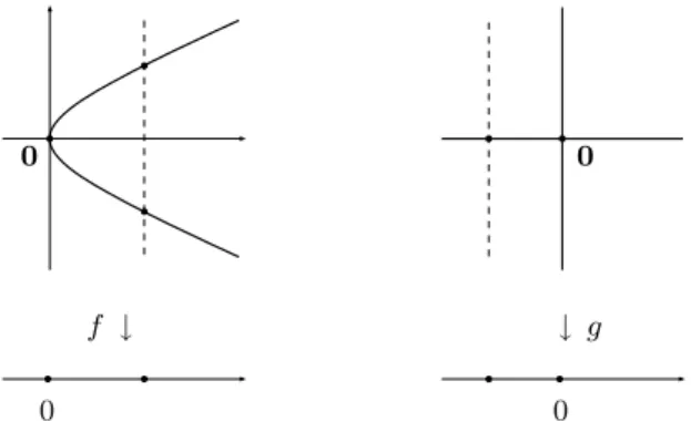
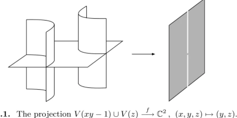
Thus, every analytic C-algebra appears as a stem of a structural sheaf of a complex space. Note, however, that the morphism of analyticC-algebrasfx is always part of the data. Let f :X→Y be a morphism of complex spaces, lety∈Y, and let x be an isolated point of the fiber f−1(y).
Then f(Z)⊂Y is an analytic subset of Y (which can be equipped with one of the structure disks in Definition 1.45). Show that f is a finite morphism and that the Fitting, annihilator, and reduced structure of the image f(X) are coincident (see Exercise 1.6.4 for a more general statement). We conclude this section with Cartan's theorem on the coherence of the full ideal sheen.
The following theorem can be understood as a diluted version of the flatness criterion (proposition B.3.5) for finite maps:. The implication (2)⇒(1) follows from Corollary 1.111 and the construction of the normalization in the proof of Theorem 1.95.
Second Riemann removable singularity theorem)
Non-reduced and non-normal locus are closed)
- Singular Locus and Differential Forms
Indeed, since the flat locus of a morphism f:X →S is analytically open by Frisch's Theorem 1.83, and since flat morphisms are open by Theorem 1.84, we can assume that f is everywhere flat and that f:X →S is surjective. In this section we characterize singular points of complex spaces and morphisms of complex spaces. Recall that it is a regular (or smooth) point of X if the local ring OX is regular (cf. Definition 1.40); is a singular point if it is not regular.
Since every isomorphismX →Y of complex spaces maps Sing(X) isomorphically to Sing(Y) (since dim(X, x) and edim(X, x) are preserved under isomorphisms), we can assume that X is a complex model space. In the following, we will give a different proof of the analyticity of Sing(X), which gives Sing(X) a canonical structure even if X is not purely dimensional. It follows that we can glue locally defined sheaves ΩU1 to obtain a unique sheaf ΩX1 on X, a sheaf of holomorphic (K¨ahler) differential or holomorphic 1-form X and a unique derivation dX:OX → ΩX1 (A.2). ΩX1 is a coherent OX-module (A.7) and satisfies
Regularity criterion for complex space germs)
Moreover, the module of relative differentials (ΩB/A1, dB/A) satisfies the following universal property: For every finitely generated module B, the linear morphism B. For a morphism f :X →S of complex spaces, we define the sheaf Ω1X/S of differential relative holomorphic (K¨ahler) forms of X over S with the correct sequence. Note that, by Proposition 1.108, the sheaf morphism:f−1OS → OX belonging to tof gives rise to a unique sheaf morphism df:f−1ΩS1 →ΩX1, which commutes with the differences f−1dS and dX. where X is the complex model space defined by the coherent ideal I ⊂ OD. 1.10.4).
Let f :X →S be a morphism of complex spaces and let x∈X. Then the following is equivalent to:. b)OX,x is a free algebra of power series over OS,f(x). Proposition 1.104 and Theorem 1.110 provide two different ways to compute the singular site of a complex space X. Another way to show that Sing(X) is an analytic subset of X (and does not use a prime decomposition) is based on Theorem 1.110, which states that.
2 Hypersurface Singularities
Invariants of Hypersurface Singularities
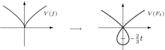
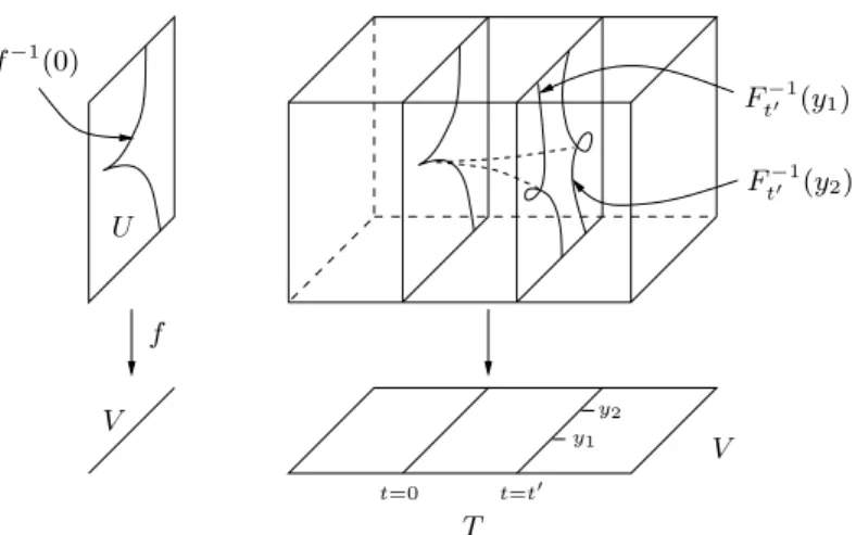
We use the notation. for the family of power series Ft∈C{x} or, after choosing a representative F:U×T →C, for the familyFt:U →Cof holomorphic functions parametrized by t∈T, where U ⊂Cn and T ⊂ Ck are open neighborhoods of the origin. The flatness of the maps φandψ follows from the flatness of the mapsφandψ (associated with F) and the basis change property for flatness (Proposition 1.87 on page 89). total". None of the corresponding hypersurfaces {fσ= 0} is singular in (C∗)2, and the truncations at the 0-dimensional planes are monomial, so hypersurfaces that have no singular point in the torus define (C∗)2 .
The right-hand side of the formula is called the mixed Minkowski volume of the polytopeK0(f), or the off Newton number. It follows that fσ has no critical point in Cn\ {0} if the hypersurface{fσ= 0} ⊂Cn has an isolated singularity at0. However, the results of the next section show that any SQH power series is equivalent to a suitable series.
Finite Determinacy
It follows that the conditions in the finite determination theorem depend only on k-jet off. However, they are close to the necessary conditions as the following supplement shows (which follows directly from Theorem 2.22). The proof is actually identical to that of Theorem 2.23, which is a special case of Lemma 2.25 withI=mk.
The following example shows that the conditions in the finite determination theorem are generally not necessarily fork-deterministic. Note that the original proof in [May] was forb= 0.1 and required f to be an isolated singularity. There is another theorem, due to Shoshitaishvili [Sho], which states that the Milnor algebra, as C-algebra, determines f to right equivalence if f is quasihomogeneous.
Algebraic Group Actions
It is affine, since it is the complement of the hypersurface defined by the determinant. Note that the somewhat unexpected multiplication in K(k) as a semidirect product (and not just a direct product) was introduced to guarantee (gh)x=g(hx) (check this out!). The following theorem about the fiber dimension of a morphism of algebraic varieties has many applications.
Then the induced mapping of local rings f#:OY,y → OX,x induces the K-linear mapping mY,y/m2Y,y →mX,x/m2X,x of cotangent spaces and is therefore its dual aK-linear map of tangent spaces. Clearly, the general case follows if we show that f(X) is constructible. Determine Tf(R(w,d)f) and calculate the number of modules in the right-hand ordering of the above sprouts.
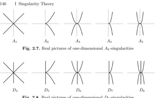
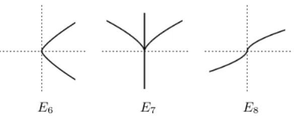
Classification of Simple Singularities
Note that for a critical point p, the rank of the Hessian matrix H(f)(p) depends only on the 2-jet off. The apparently simple proof uses the finite determination theorem (Theorem 2.23, which required a little work). Then there exists a linear automorphism ϕ∈C{x, y} such that f(3), the3-jet iϕ(f), is of one of the following forms. 1)xy(x+y)or, equivalently,f(3) factors into 3 different linear factors, (2)x2y or, equivalently,f(3) factors into 2 different linear factors,.
After a linear change of coordinates we get a homogeneous polynomial of the same type, but meta= 0. In the latter case, for any power series g close to f, the 3-ray must factor g(3) into 2 or. 3 different linear forms, since this is an open property (by continuity of the roots of a polynomial, cf. the proof of Theorem 2.50). Algorithmic classification of ADE singularities. The proof of the classification of the simple singularities is effective and provides a concrete algorithm to decide whether a given polynomial ∈m2⊂C{x1,.
3 Plane Curve Singularities
Parametrization
If (C,0) decomposes into several branches, then the aparametrization of (C,0) is a system of branch parameterizations. The main result of this section is the following generalization of the implicit function theorem for convergent or formal power series. Indeed, the Galois group of the field extension K= Quot(Cx)→Quot(Ct) =L, x →tm consists of the mth roots of unity and Π ∈L[y] is invariant under this group.
The main tool for Newton's algorithm to compute a parametrization for a branch of the singularity of a plane curve is the Newton diagram Γ(f) :=Γ(f,0) of f at0 (cf. Definition 2.14 ). In addition, f is conveniently called if the Newton diagram satisfies the coordinate axes, that is, there exists a positive integer such that (k,0),(0, )∈supp(f). Proof of Theorem 3.3. It suffices to show that the (infinite) Newton-Puiseux algorithm 3.6 is well defined and returns a power series.
Intersection Multiplicity
Then there exist open neighborhoods of the origin, D⊂C and B ⊂C2, and a holomorphic representationϕ:D→B for the parameterization such that. 17 Instead of using the finite coherence theorem, we could use the singularity resolution of the plane curve with inflation (as presented in section 3.3) and the recursive formula (3.3.2) for the intersection multiplicities of strict transformations, cf. Example 3.14.1. Let's re-examine the multiplicity of the intersection of the regular cord (f =x2−y3) with the smooth germs of the curve given by x and αx+y, respectively.
Since 0 is an isolated point in the intersection V(f)∩V(g) inU, we can assume (after shrinking U if necessary) that it is indeed the unique intersection of the curves C and D inU. 18 A priori it is clear that for N sufficiently large, the N beam of the parameterization is sufficient to calculate the intersection number. Show that the intersection multiplicity of f and gi is at least the product of the respective multiplicities, i.e.
Resolution of Plane Curve Singularities
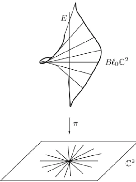
We call BzM →M amonoidal transformation inflatingz∈M, or simply inflating the pointz∈M. 3). In particular, we can define the inflating of the seed (M, z) at z as the seed of π:BzM →M along E=π−1(z) (that is, an equivalence class of morphisms defined on a neighborhood of E ⊂BzM). Blowing up curves and germs. Below we study the effect of inflating π:BzM →M on a curveC⊂M.
Note that the total transformation of the curve germ (C, z) is not a curve germ, but the iCalong E germ, while the strict transformation of (C, z) is a germ set of plane curve singularities. The intersection of the strict transformation C with E consists of at most m points given by the local equations. The disconnected tangents are in 1–1 correspondence with the intersection points of the strict transformation Cof (C,0) with the extraordinary divisor E (cf.