Accurate knowledge of the sediment budget of a coastal cell is necessary for coastal management and the prediction of long-term coastal changes. Doing so requires a solid understanding of sediment sources and sinks for a given coastal cell. An important component of the sediment budget, which is often poorly constrained in rocky and entrenched coastlines, is related to sediment transport around the folds that limit coastal landslides, defined as landward bypass [3,4].
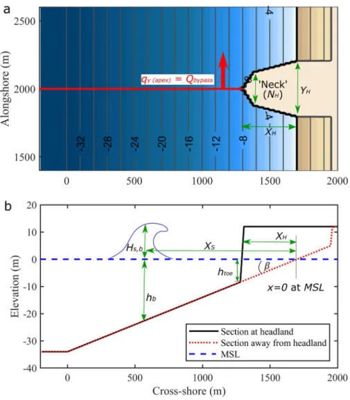
The results (Section 3) begin with the calibration of the open-shore current expression for use with XBeach (Section 3.1), followed by the determination of the expression for predicting bypass rates (Section 3.2), including the impact of changing cape shape (Section 3.3) and changing refractive index (Section 3.4). For equilibrium concentration, sediment mixing is a function of the Euler mean velocity, the infragravity velocity, and the orbital velocity of the waves (Soulsby, [29]). For all model scenarios, a domain of 3 km along the coast (y, positive to the top of the site) and 2 km across the coast (x, positive land) was used, with the top of the grid marked as 'north'.
The XBeach grid optimization function in the XBeach Matlab Toolbox [30] was used with a minimum grid size of 10 m at the coastal position of the cape. The “instantaneous” bypass velocity was determined as the longshore current for the transect from the tip of the cape (Figure 2), time averaged from 𝑡 = 60 to 90 min. If the neck is set to <100% of the cross-shore extent, the headland tapers to a point at the top of the headland.
The XBeach estimates of flux past the head were then compared to the prediction of the bypass expression.

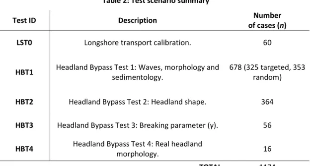
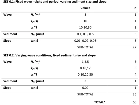
Results, applications and validation 1 Longshore transport formulation (LST0)
For the intermediate case, where the break occurs just within the fold extension (Fig. 5—middle row), a significant offshore diversion of current and sediment flux occurs (Fig. 5f,g,h). The flux is significantly reduced ( Fig. 5h ), however it is still a significant fraction of the open coast flux (blue and red lines in Fig. 5h ). For the extreme energy case, where fracturing occurs well offshore of the crest (Fig. 5—bottom row), there is a small offshore deviation of sediment velocity and flux (Fig. 5j,k,l) , but the total flow along the coast at the top is similar to the rates of the open coast (Fig. 5l).
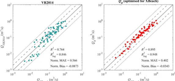
The XBeach predictions of instantaneous flux past the headland tip (𝑄 ) for each targeted case in HBT1 (Table 4, n = 325) are first compared to the calibrated open coast (i.e. no headland) alongshore sediment transport parameter (𝑄 ) ( Fig. 6a ) . However, in many of the cases, 𝑄 ≫ 𝑄 (top left in Fig. 6a) and in these cases the headland limits the flux. Exploring this relationship further, 𝐵 is plotted against the modeled alongshore flux past the foreland for a fixed wave height and angle (Fig. 6b).
This approach was tested against all the input variables (Fig. 7) to ensure that the expression (𝑄 , ) is not systematically biased relative to any of the inputs. The combination of headland cross-coastal extent (𝑋 ), along-shore extent at the shoreline (𝑌 ) and “neck” ratio (𝑁 ) was used to generate all the headland landforms in this study (see methods: Fig. 2a , Section 2.3.3). However, there is no consistent pattern in the distribution of the head shape (compare Fig. 9b and 9d).
Sediment transport around the crest was allowed to occur only below this depth (colored area outside the crest in Fig. 11b). The effect of the shoal in reducing the open coast flux rates is evident ( Fig. 11c ), with the 𝑄 bias increasingly overestimated as the wave height decreases. There was good agreement between the XBeach estimates and the hip bypass parameter in most cases (Fig. 11d), with the parameter being within a factor of two of the XBeach norms for most cases, clearly demonstrating the utility of the expression.
The headland variables are then linearly interpolated to a water level time series (Fig. 12b), using the tidal coefficient for each time step (0 = mean spring low water level, 1 = mean spring high water level). One of the few observational studies of bypass was made at Start Bay, UK, over an easterly storm cluster in Feb-Mar 2018 (Fig. 13a-b; details in [20]). The dimensions of the headland were estimated by drawing an 'upward coastline' and extracting a cross-section of the land (Fig. 13, rows 3-4; using the method in Fig. 1).
A time series of the ratio of the oscar length to the width of the wave zone (𝑋 /𝑋 ; for the central values given in Fig. 13f-h) and the potential current (𝑄 ) is given for each of the three oscars (Fig. 13, i-k ). The ratio 𝑋 /𝑋 shows clear tidal fluctuations, with the length of the headland increasing with each high tide and decreasing 𝑋 /𝑋 above the peak of 𝑄 around 02/03/2018, e.g. Cape 1 (Fig. 13l). ) at this time is mostly within the surf zone (𝑋 /𝑋 < 1).
Discussion
The length of containment buoyancy of a headland or structure determines whether the flow along land has room to develop fully. In comparison, the conceptual model of "embayed beach state" [3, 39] categorizes bays according to the number of surf zone widths that fit into the embedment length (𝛿 = 𝐿/𝑋. For 𝛿 ≥ 20, beaches generally exhibit 'normal' circulation, where more rip -channels can be observed along the beach.
We suggest that the bypass parameter can be used if the beach is in a normal configuration, with sufficient space for the development of the coastal current [21]. In cases where the length of the bay is short relative to the surf zone (𝛿 < 10), a strong geological control of the flow can be exerted, resulting in "cellular circulation in the bay", with the occurrence of mega-rips [40]. ]. An extension of levee-scale circulation behavior is "multi-levee circulation" [10], which refers to the changes in flow behavior that occur on levee banks during extreme wave conditions when breaking occurs far offshore of smaller headlands and the levee boundaries are newly defined.
The extent of smaller headlands becomes insignificant relative to the width of the wave zone, and circulation becomes a function of wave interactions with distant headlands. Such effects are predicted to be highly non-linear with possible flow reversals (Section 3.4). This phenomenon is predicted by numerical models but not observed in the field.
Until further research is available in this area, we recommend that when using the bypass parameter, you check whether: (i) breakage occurs near or outside the range of interest, or If both conditions are met, multibay circulation effects may occur that will not be accounted for by the bypass term. There are limited observations of currents around headlands, but there are direct measurements of sediment transport or changes in bottom elevation.
13] or have widely dispersed temporal resolution [9], making it difficult to determine instantaneous rates of sediment flux under extreme conditions when the bulk of the bypass is expected to occur. The observations of [20] used for validation in Section 3.7 are an exception, although even these are limited to before and after a single storm event. The bypass expression generated in this study will need to be tested and refined against additional field data if and when these become available.
How to apply the bypassing expression
Conclusions
ACKNOWLEDGEMENTS
The influence of wave, wind and tidally forced currents on headland sand diversion – Case study: Santa Catarina Island north coast, Brazil. Dynamics of rip currents associated with reefs—field measurements, modeling and implications for beach safety. Physical model study of beach profile evolution due to sea level rise in the presence of seawalls.