Assessing the validity of regular wave theory in a short physical wave flume using particle image velocimetry

(1)

University of Plymouth

PEARL https://pearl.plymouth.ac.uk

Faculty of Science and Engineering School of Engineering, Computing and Mathematics

2021-02-01

Assessing the validity of regular wave theory in a short physical wave flume using particle image velocimetry

Windt, C

http://hdl.handle.net/10026.1/16529

10.1016/j.expthermflusci.2020.110276 Experimental Thermal and Fluid Science Elsevier

All content in PEARL is protected by copyright law. Author manuscripts are made available in accordance with publisher policies. Please cite only the published version using the details provided on the item record or

document. In the absence of an open licence (e.g. Creative Commons), permissions for further reuse of content should be sought from the publisher or author.

(2)

Assessing the validity of regular wave theory in a short physical wave flume using particle image velocimetry

Christian Windt^a,∗, Alix Untrau^c, Josh Davidson^b, Edward J. Ransley^d, Deborah M. Greaves^d, John V. Ringwood^a

aCentre for Ocean Energy Research, Maynooth University, Co. Kildare, Ireland

bDepartment of Fluid Mechanics, Faculty of Mechanical Engineering Budapest University of Technology and Economics, Hungary

cInstitut National Des Sciences Appliqu´ees, Lyon, France

dSchool of Engineering, University of Plymouth, UK

Abstract

The modelling of ocean waves is an integral part of coastal and offshore engineering. Both theoretical and experimental modelling methods are available and are commonly used in support of each other. In particular, due to the difficulty in measuring the velocity throughout the water column, the wave kinematics are often derived, by means of wave theory, from a measurement of the free surface elevation. However, wave theory is often based upon idealistic conditions, such as infinite spatial domains and time lengths. The question therefore arises, how well are the wave kinematics in an experimental wave tank described by wave theory? The present paper compares theoretical solutions against experimental data, for the free surface elevation and the velocity throughout the water column, to assess the ability of Stokes’ wave theory to describe the kinematics of regular waves in a short, physical, wave flume. Experimentally, the free surface elevation is measured with a set of resistive wave probes, while wave kinematic data is acquired with particle image velocimetry (PIV). For this study, ten different regular waves, of varying steepness, are generated in a 35m long and 0.7m deep wave flume. The theoretical solutions are computed based on Stokes 2^nd order wave theory. The presented results show error values of the order of 10–20%, indicating validity of the employed wave theory as a function of the reflection coefficient achieved in the physical wave flume. These result highlight the potential inaccuracies incurred in any wave tank if the wave theory is used to derive the kinematics from the free surface elevation without having detailed knowledge of the reflection characteristics at the point of interest in the tank.

Keywords: Wave kinematics, Regular waves, Wave theory, PIV, Physical wave flume

∗Corresponding author

Email address: [email protected](Christian Windt)

(3)

1. Introduction

Waves transport energy, via oscillations of the air-water interface, in the Earth’s vast oceans and coastal areas. The energy carried by waves is of the order of 40–60kW m⁻¹, for over 70% of the Earth’s surface [1]. The large mass density of water (1000 times greater than air), and the large spatial area which the energy transfer from the wind to the ocean is integrated, results in enormous amounts of momentum transported by the waves. Understanding and modelling the kinematics of water waves is, therefore, important in fields such as coastal protection [2], naval architecture [3], offshore oil and gas [4], and marine renew- ables [5]. For example, Gudmestad [4] highlights the importance of the accurate description of the wave kinematics, stating that the use of different kinematic models, can lead to differences of up to 75% in the estimated load on offshore structures.

1.1. Wave analysis

Analysis of wave kinematics and wave structure interaction (WSI), is commonly performed based on experimental data or theoretical models and their analytical/numerical solution. Physical wave tank experiments provide a real world truth. The laboratory environment allows substantial benefits compared to testing in the open ocean, in terms of: (1) control of the experiment param- eters, (2) ability to repeat experiments, (3) relatively low cost, and (4) ability to conduct frequent calibration of the measuring instruments. However, while measurement of the free surface elevation (FSE) is relatively simple and inex- pensive, obtaining physical measurements of the velocity throughout the water column is significantly more challenging. Due to the relative difficulties involved in directly measuring the wave kinematics, a common approach is to derive the velocity values, throughout the water column or at points of interest, using wave theory based on the measured FSE.

Numerical wave tanks (NWTs) are commonly used in the field of ocean and coastal engineering [6–10], providing several advantages to testing in physical wave tanks, in terms of: (1) cost, (2) access and availability, (3) the ability to limit reflections from the tank walls, and (4) the ability to non-intrusively measure any variable at any location. The main disadvantage of NWTs is the requirement for validiation against experiments before the simulation results can be fully trusted. Wave theory is also employed in NWTs, through the numerical wave makers, used to generate and absorb the waves into/out of the tank. The numerical wave makers are generally based on algorithms employing a theoretical description of the wave kinematics (i.e. wave theories) [11, 12].

Wave theory, therefore, plays an important role across the range of experimental and theoretical analysis methods for water waves. Three main ap- proaches are employed to describe ocean waves: (1) regular waves, consisting of a monochromatic representation of the water surface, (2) irregular waves, comprising the summation of a finite number of harmonics, and (3) a full spectra, containing an infinite summation of Fourier components [13]. Thus, regular waves provide the basic building block upon which more realistic and complex

(4)

descriptions of ocean waves can be derived [14]. Several theories have been developed to mathematically describe the kinematics of regular waves. Wave theories such as Stokes [15], Cnoidal [16], and Fourier [17] are commonly applied in analyses [18]. However, in addition to assuming the fluid to be inviscid and irrotational, such wave theories are generally derived under the simplifying assumption of infinite spatial and temporal domains.

Given that physical wave tanks are inherently of finite length, it is important to understand the limitation of wave theory in describing the kinematics within a wave tank. Sobey [19], for instance, states that laboratory measurements of regular waves are notoriously irregular due to the influence of harmonic contamination from the wave maker, reflections from the beach and the wave maker, resonant modes within the flume, and bound long wave motions, all of which violate the basic assumptions of steady wave theory.

1.2. Comparison of theoretical wave kinematics with wave tank measurements The comparison of wave theory to measurements of the fluid velocity in a physical wave tank has been performed for a range of scenarios, such as: bichromatic waves [20, 21], irregular waves [22–26], extreme waves/focused waves [27–33], internal waves [34–36] and the investigatioon of the higher order drift effects [37–41]. Considering the fundamental case of regular waves, several studies can be found in the literature performing experimental measurements of the wave kinematics and comparing the results to wave theories.

The earliest studies predominately utilised Laser Doppler Anemometry (LDA) [42] measurements at several points within the wave column for comparison against theory. Swan [43], motivated by wave loading, focuses on the wave kinematics just beneath the wave crest. The comparison with established wave theories shows “a very good description” of the wave kinematics by steady wave theory when Eulerian back–flow is included. Zhanget al. [44] compare the measured wave kinematics of regular and dual component wave trains against linear wave theory, finding good agreement. Kim et al. [28, 29], during the investigation of extreme/rogue waves, also perform tests of a large regular wave for comparison and compare the results with Stokes 3^rd order wave theory, finding good agreement when Wheeler stretching is included. In addition to irregular waves, Choi et al. [25] also consider regular waves, comparing the results of the horizontal velocity under the wave crests against linear theory and a fully nonlinear NWT, finding that the NWT more closely matches the experimental data. From the results, Choiet al. deduce a negative mean flow when a positive mean flow would be expected from the second-order Stokes wave theory.

The main limitation of the LDA method, is that it provides a point measurement only, requiuring the LDA to repositioned in multiple repeat tests to gather kinematic data throughout the water column. The more modern studies therefore favour Particle Tracking Velocimetry (PTV) [45], which allows the visualisation of particle paths, and Particle Image Velocimetry (PIV) [46], which provides velocity field data in a defined interrogation window. Choi [47] per- forms both LDA and PIV experiments for regular waves, finding agreement between the two methods. Examining the measured velocities under the wave

(5)

crest, Choi finds that the velocity magnitude may correlate with the wave elevation, however as the wave slope increases the ability of 3^rd order Stokes theory to match the data decreases.

As part of their PIV investigation into the kinematics of rogue waves Choiet al. [33, 48] and Jung et al. [32] also perform tests of a large regular wave for comparison. unlike the majority of other studies, the quality of the incoming wave field is quantified, providing the root-mean-square error between the wave height of consecutive wave periods and the mean wave height. Error values of less then 1% suggest good consistency of wave propagation. For the velocity profiles, overall good agreement between the phase-averaged experimental data and 3^rd order Stokes theory is found, with the errors increasing for the waves with larger slopes to a maximum value of 9.6%.

Jensenet al. [49] present a two-camera PIV system to measure the acceleration field for a range of wave lengths and heights, representing deep and finite depth conditions. Comparing the results against linear wave theory, qualitatively good agreement is found. A quantitative assessment is only presented for the scatter in the experimental data, using the relative standard deviations as a metric. An analysis of the surface elevation data is omitted in the study and only the measurement uncertainty in the wave probes (3%) is stated. Kris- tiansenet al. [50] perform PIV measurement for propagation of regular waves as well as wave diffraction due to the interaction with a fixed cylinder, specifically for the purpose of CFD validation. Generally, good qualitative agreement between the physical measurements, linear wave theory, and CFD is found for the wave propagation test cases. Umeyama [37] utilises PIV to investigate the trajectory of water particles under a wave. Satisfying agreement is found in the qualitative comparison of the measured horizontal and vertical velocity under a crest, trough and zero-crossings, against third-order Stokes wave theory.

The same author presents coupled PTV and PIV measurements for regular waves, with and without a current in [51]. The measured FSE and the wave kinematics are compared to 3^rd order Stokes wave theory, finding good agreement qualitatively. Grueet al. [52] investigate the kinematics near the breaking limit, using PTV measurements. Comparison of the results against calculations based on Fenton’s method [53], reveal that the measured waves display a large degree of asymmetry compared to the theoretical wave with perfect symmetry.

1.3. Objectives and motivations of the present paper

The objective of the present paper is to assess the ability of Stokes wave theory to describe the wave kinematics of swell waves, based on measurement of the FSE, in a short physical wave flume. The motivation for specifically considering a short wave flume is to enable the applicability of the results to practical wave tank testing situations, in which the finite length of the tank has a non-negligible effect on the wave kinematics. While several studies have investigated the ability of wave theory to describe the wave kinematics measured in a physical wave tank, they have done so under ideal conditions, performing the measurements close to the wave maker, utilising a long enough wave tank and short enough time window to eliminate the effect of reflections [33, 48, 49].

(6)

However, in many practical cases, the experiment can not fulfil these criteria, since the testing location in the tank may be set by other requirements (e.g. the position of a gantry) or the duration of the experiment may need to encompass many wave periods.

Given that, in the vast majority of testing campaigns, the only measurement of the wave kinematics is the FSE, from which velocity data must be inferred from wave theories¹, there is a clear motivation to assess the validity of this approach in realistic experimental conditions. Indeed, the problem of estimating the velocity data in the water column from a measurement of the FSE is explored in Johannessen [55], for irregular waves and focussed wave groups; however, no reflection analysis is presented in [55]. Likewise, although some of the studies reported in Section 1.2 do not consider the ideal conditions of testing in long tanks for short durations, the analysis of the reflection characteristics of the wave tank is either omitted entirely or very limited and generalised. For example, [37]

states that the wave absorber “limited the reflection to 5 per cent over a wide range of water depth, wave period and wave height.”

The contribution of the present study is to provide a rigorous measurement of the reflection coefficient for each individual test, and investigates through quantitative analysis, the effect which this has on the measured kinematics for regular waves. The provision of a quantitative analysis represents another gap in the literature which the present study aims to fill, with the majority of existing comparisons between wave theory and measurements of the wave kinematics performed on a qualitative basis only. The present study considers a set of 10 regular waves, with varying steepness and water depth conditions. After performing both reflection and repeatability analyses for the considered regular waves, the experimental FSE and kinematics data are compared to wave theory.

The remainder of the paper is organised as follows. Section 2 describes the experimental test campaign. Section 3 introduces the wave theory used for the comparison with the experimental data. The results of the comparative analysis are then presented in Section 4. Finally, conclusions are drawn in Section 5.

2. Experimental study

The physical wave tank setup is detailed in this Section. Section 2.1 describes the wave flume, Section 2.2 provides information on the measurement equipment, i.e. the wave probes and the PIV system. Section 2.3 then introduces the test matrix of the experimental test campaign.

2.1. Physical wave flume

The experiments were conducted in the 35m long and 0.6m wide wave flume in the COAST laboratory at the University of Plymouth, UK. For the present study, the water depth in the flume is set to 0.7m. The wave flume is equipped

1Although interestingly, one recent paper attempts to do the opposite and estimate the FSE from velocity measurements [54]

(7)

with an Edinburgh Designs Ltd. (EDL) piston-type wave maker. An absorbing beach, constructed from wave-absorbing foam, is installed towards the end of the wave flume. A photograph of the experimental test facility and a 3D schematic of the beach is shown in Figure 1. A schematic of the experimental set-up including all relevant measurements is given in Figure 2.

High-speed camera Wave probes

High-speed camera

Wave probes

Figure 1: Photograph of the wave flume, showing the high–speed camera for the PIV measurements and the wave probes, looking down-wave towards the beach (a) and up-wave towards the wavemaker (b). Top view photograph of the absorbing beach (c) and a 3D schematic of the beach set-up (d).

2.2. Measuring equipment

Resistive wave probes are used to measure the FSE. A PIV system is employed for measurement of the water particle velocities.

2.2.1. Resistive wave probes

Eight commercially available, resistive EDL wave probes [56] (labelled WP in Figure 2) are located in the tank. The probes are constructed of two parallel vertical wires, immersed in water. The electrical conductivity between the two wires correlates linearly with their depth of immersion, allowing the measurement of the FSE. For this study, an accuracy of±0.5mm is assumed for resistive wave probes. A five–point calibration method, with 0.05m steps, was used re- peatedly throughout the test campaign to calibrate the wave probes. For more

(8)

3.210 3.210

16.963

0.7

32.916

0.482 0.136

0.204

0.321

(a) Side view

(b) Top view

0.6

0.15

2.500 Wave

paddle

Figure 2: Schematic of the wave flume with the main dimensions in [m]. Eight wave probes, labelled WP, are located in the tank. Wave probe 3 is located at the centre of the PIV interrogation window (green colour coded rectangle). An absorbing beach is installed at the end of the wave flume, opposite the wavemaker (yellow colour coded triangle).

details on the specifications of the wave probes, the interested reader is referred to [56].

Wave probes 1 and 2, closest to the wavemaker paddle, are located at the same horizontal distance from the wavemaker (i.e. 16.69m). Wave probe 1 is located on the centre line of the wave flume, while wave probe 2 is installed off centre, to identify any inconsistencies in the along-crest direction. The remaining wave probes (3–8) are all aligned with wave probe 1, along the centre line of the wave flume. Wave probe 3 is located at the centre of the PIV interrogation window (green colour coded rectangle in Figure 2). Wave probes 4–8 are installed for the determination of the reflection coefficient within the wave flume.

2.2.2. Particle image velocimetry

PIV allows the instantaneous horizontal and vertical velocities in the water flow to be measured, using sequential pairs of images of small tracers suspended in the water, recorded by a high-speed camera [57]. A thin sheet of laser light illuminates the flow over a defined area, to ensure good visualization of the tracers.

In this study, time resolved PIV is employed, where velocity measurements are taken over a temporal interrogation window of of five consecutive wave periods. A single camera, a VDS Vossk¨uhler CMC-4000, with a frame rate of up to 400 fps and a resolution of 2320×1726 pixels [37] is used for this study.

A Nd:YAG laser Litron NANO L 50-100 [38] is used to illuminate the flow

(9)

field. The calibration, data logging, and post-processing is performed with the Dantec DynamicStudio software [39]. For the calibration, the DantecDynamic software prescribes a standardised procedure, ensuring the correct alignment of the camera with the laser sheet.

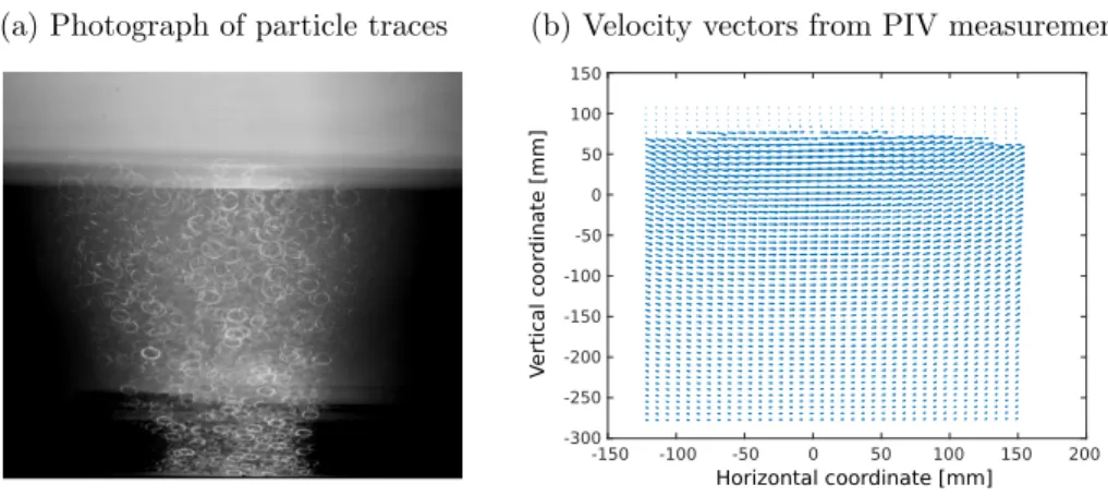
In this study, the interrogation window spans 270mm in the wave direction (horizontally) and 382mm perpendicular to the wave direction (vertically). The image field is divided into 64×64 pixel interrogation windows. In each interrogation window, a cross-correlation analysis between the two images of a pair is performed to determine the velocity field data. After post-processing, velocity vector fields (see Figure 4 (b)) with a spatial resolution of 37×52 vectors in the horizontal and vertical direction are generated every 0.04s within the temporal interrogation window.

-150 -100 -50 0 50 100 150 200

-300 -250 -200 -150 -100 -50 0 50 100 150

Horizontal coordinate [mm]

Vertical coordinate [mm]

Figure 3: Example photograph of the particle trajectory during the PIV experiment, recorded with a DSLR camera with long exposure (a) and an example velocity vector field, post- processed from the PIV data (b).

2.3. Test matrix

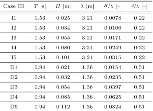
Ten different regular waves are considered in this study. The waves can be clustered in two groups of different wave periods, T, and corresponding depth conditions. Waves I1–I5 are inspired by [51] and have a wave period of 1.53s, resulting in a wave lengthλof 3.21m and, thus, intermediate water conditions at the tested water depth of 0.7m. The wave height parameter space has been extended in this study, compared to [51], to cover a wider range of Stokes 2^nd order theory. To also cover deep water conditions and, thus, comply with the assumption in the wave theory, waves D1-D5 have a wave period of 0.94s, resulting in a wave length of 1.36m. The wave height, H, varies from 0.024m, for the smallest wave, to 0.144m, for the largest wave. The characteristics (i.e.

T, H, wave length,λ, wave steepness,^H/λ, and water depth over wave length,

d/λ), for the individual waves, are listed in Table 1.

(10)

Table 1: Wave period,T, wave height,H, wave lengthλ, wave steepness,^H/λ, and wave depth over wave length,^d/λ, of the ten considered regular wave test cases

Case ID T[s] H[m] λ[m] ^H/λ[–] ^d/λ[–]

I1 1.53 0.025 3.21 0.0078 0.22

I2 1.53 0.034 3.21 0.0106 0.22

I3 1.53 0.055 3.21 0.0171 0.22

I4 1.53 0.080 3.21 0.0249 0.22

I5 1.53 0.101 3.21 0.0315 0.22

D1 0.94 0.021 1.36 0.0154 0.51

D2 0.94 0.032 1.36 0.0235 0.51

D3 0.94 0.054 1.36 0.0397 0.51

D4 0.94 0.085 1.36 0.0625 0.51

D5 0.94 0.112 1.36 0.0824 0.51

3. Wave Theory

For linear, regular waves, which are sinusoidal in nature, the following conditions must hold; (1) Small amplitude (relative to the wave length), and (2) Intermediate to deep water (water depth/wavelength≥0.05). The relevance of these two conditions can be observed by the location within the Le M´ehaut´e diagram [58] where linear wave theory is valid (see Figure 4). Under these physical conditions, the FSE and the wave kinematics, are analytically well described by linear wave theories, such as: 1^st order Stokes theory [15]. Beyond these ideal conditions, the wave kinematics become nonlinear, with the nonlinearity increasing in prevalence for larger wave height and steepness, as well as towards shallow water conditions. For these larger waves or in shallow water conditions, the linear assumptions are violated, resulting in inaccurate solutions from linear wave theory. Higher order Stokes’ wave theory extends linear wave theory, better describing the kinematics of nonlinear waves up to the breaking limit.

The nonlinearity of the wave kinematics also increases with the proximity to the free surface, especially for the crest phases [59]. However, the analytical solutions of the wave kinematics are linearised around the mean water level and do not readily provide solutions within the wave crest [19, 51]. To calculate the solutions for the wave kinematics within the wave crest, as well as underneath the wave trough, for nonlinear waves, additional models have been developed, such as Wheeler stretching or linear extrapolation techniques [3] (see Section 3).

For the present study, the set of 10 regular waves listed in Table 1 are located on the Le M´ehaut´e diagram in Figure 4). It can be seen that the considered regular waves fall within the range of Stokes 2^nd and 3^rd order wave theory.

Investigating the difference between the results from Stokes 2^nd and 3^rd order wave theory for the two 3^rd order waves, i.e. D4 and D5, negligible differences (approx. 1%) between the theoretical FSE profiles are found. Thus, in the following, only Stokes 2^nd order is considered for the comparative analysis of the experimental results and wave theory. This section gives a brief overview of

(11)

Stokes 2^nd order wave theory for both the FSE and the wave kinematics.

I I I I I D D D D D

Figure 4: Location of the tested regular waves in the Le M´ehaut´e diagram [58]. H denotes the wave height,T the wave period,gthe gravitational acceleration, anddthe water depth.

3.1. Free surface elevation

Under the assumptions of inviscid and irrotational fluid in an infinite domain, the FSE,η⁽¹⁾(t), of a linear, first order Stokes wave at a given location xcan be described by:

η⁽¹⁾(t) =a·cos(θ), (1)

whereadenotes the wave amplitude. θdenotes the phase functionkx−ωt, with the wave numberk=^2π/λ, the space variable in wave propagation direction x, and timet. With increasing wave height and steepness, linear, first order wave theory can be extended, from Equation (1), to capture non-linear effects, using 2^nd order Stokes wave theory, which describes the FSE as:

η⁽²⁾(t) =η⁽¹⁾(t) +πH² 8λ

cosh(kd)

sinh³(kd)·[2 + cosh(2kd)] cos(2θ), (2) whereddenotes the water depth.

3.2. Velocity profiles

Based on the FSE, the velocity profile in the water column can be obtained from Stokes wave theory. For first order linear waves, the horizontal,u⁽¹⁾, and vertical velocities,v⁽¹⁾, follow:

u⁽¹⁾(z) = πH T

cosh(k(z+d))

sinh(kh) cos(θ) (3)

(12)

v⁽¹⁾(z) = πH T

sinh(k(z+d))

sinh(kh) sin(θ), (4)

where z denotes the vertical depth within the water column, with negative z values towards the sea floor. Extending the description of the wave velocity to second order, delivers:

u⁽²⁾(z) =u⁽¹⁾(z) +3 4

πH T

πH λ

cosh[2k(z+d)]

sinh⁴(kd) cos(2θ) (5) v⁽²⁾(z) =v⁽¹⁾(z) +3

4 πH

T πH

λ

sinh[2k(z+d)]

sinh⁴(kd) sin(2θ). (6) Due to linearisation around the free surface, the descriptions of the horizontal and vertical wave velocities, delivered by Stokes wave theory, are only available up to the still water level. Additional theoretical models, such as extrapolation or stretching, have to be used to describe the in-crest velocities [3].

Employing the linear extrapolation technique, the values for the horizontal and vertical velocities are calculated up to the still water level. Within the wave crest, the velocity at the still water level is then extrapolated, to accommodate positive values ofz.

Using the Wheeler stretching method, proposed in [60], a new vertical coordinate,zs(t), from the sea floor to the free surface,−d < zs(t)< η(t), is defined.

Following Equation (7),zs(t) can be related to thez coordinate lying between

−d < z <0, which is then substituted in Equations (3)–(6).

z=zs(t)−η(t)

1 +^η(t)/d (7)

While the linear extrapolation method does not alter the velocity profile below the still water level, compared to linear wave theory, Wheeler stretching implies changes to the velocity profile over the entire depth of the water column. The influence of extrapolation and Wheeler stretching is illustrated in Figures 5 (a) and (b), showing the horizontal velocity profiles underneath the wave crest and trough, for the regular waves I1–I5 (a) and waves D1–D5 (b), for extrapolation (solid lines) and Wheeler stretching (dashed lines).

(13)

Intermediate water conditions

I I I I I

Deep water conditions

D D D D D wave crests wave troughs

wave crests wave troughs

Figure 5: Horizontal velocity profiles, using velocity extrapolation (solid lines) and Wheeler stretching (dashed lines), underneath crests (v⁽²⁾>0) and troughs (v⁽²⁾<0), for waves I1–I6 (a) and D1–D5 (b).

4. Results and discussion

This section presents the analysis of the experimental results. Section 4.1 details the results of the reflection analysis, with Sections 4.2 and 4.3 presenting the analysis of the FSE and velocity data, respectively. A discussion of the results is provided in Section 4.4.

4.1. Wave reflection

The efficient absorption of waves, to eliminate contamination due to reflections from the tank end wall, is crucial for the replication of open ocean conditions in a physical wave flume. To assess the wave absorption effectiveness within the test facility, for a specific wave, the reflection coefficient,R, can be calculated, which is defined as the ratio between incident and reflected wave

(14)

spectra¹. Following Mansard and Funke [61], Ris calculated following R=

SˆηR

SˆηI

·100%, (8)

where ˆSηI is the peak value of the spectral density of the incident wave at a frequencyfp. ˆSηRis the spectral density of the reflected wave atfp. To separate the incident and reflected wave field, a three point method is proposed in [61], where the FSE time traces are measured at three different wave probes, spaced at specific relative distances from each other. Based on the guidelines provided in [61], the distance between the first and the second wave probes is ^λ^p/10, and the distance between first and the third wave probes is^λ^p/4. Accordingly, WP4 – WP6 are considered for the determination of the reflection coefficient for waves D1–D5, while WP6 – WP8 are considered for waves I1–I5. The reflection coefficient results for all waves are listed in Table 2.

Table 2: Reflection coefficients for waves I–I5 and D1–D5

Case ID Reflection coefficient [%]

I1 11.6

I2 12.4

I3 14.5

I4 16.8

I5 18.5

D1 7.3

D2 7.5

D3 8.2

D4 9.1

D5 13.8

4.2. Free surface elevation

Here the FSE measurements are analysed, first in terms of repeatability, in Section 4.2.1, and then by comparison with wave theory, in Section 4.2.2. For the analysis, the FSE data from WP3 is considered, whose location coincides with the centre of the PIV interrogation window.

1Note that the reflection coefficient varies between 0% and 100%, where 100% refers to full reflection and 0% to full absorption

(15)

4.2.1. Repeatability

Repeatability considers if the regular wave is identical between consecutive wave periods of the same experimental run and between different experimental runs. Phase averaged FSE data is utilised to assess repeatability, following the phase averaging procedure demonstrated in [12]. The FSE signal is broken into individual wave periods, then the FSE value at each phase of the wave cycle is averaged across individual wave periods.

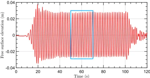
The entire FSE signal is not utilised to assess repeatability, rather a temporal interrogation window is manually selected, which exhibits a steady–state–wave time trace. Any remaining unsteady characteristic of the FSE trace is accounted for in the phase averaging procedure by means of the standard deviation, σ, between consecutive periods. By way of example, Figure 6 shows the time trace of the measured FSE (at WP3), for wave I3, with the interrogation window for the phase-averaging procedure framed in blue.

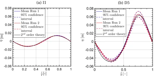
Illustrative examples of the phase-averaged FSE, for waves I1 and D5 (the least and most steep amongst the considered waves) are shown in Figures 7 (a) and (b), respectively. The figures show the mean, phase-averaged FSE (solid line) ± the 95% confidence interval² (dashed line). Furthermore, results for two independent experimental runs of the same wave are plotted (blue and red colour coded)³.

Figure 6: Complete time trace and for case I3. The interrogation window for the phase- averaging procedure is frame in light blue.

295% confidence interval = 1.96σ, whereσdenotes the standard deviation

3Note that Figures 7 (a) and (b) also include time traces for the solution of the free surface elevation based on 2^ndorder Stokes wave theory. In this section, no comparison between the experimentally measured data and the theoretical solution is undertaken. For the comparative analysis see Section 4.2.2.

(16)

(a) I1 (b) D5

Figure 7: Wave elevation repeatability for case (a) I1 and (b) D5

Analysing the repeatability between the two independent experimental runs, close agreement can be observed in Figures 7 (a) and (b), where the results for the two runs virtually overlay each other. The high repeatability negates the requirement to perform multiple runs of each experiment; thus, only data from a single run are considered for the following analyses.

Regarding the repeatability of the FSE between consecutive periods, the 95% confidence interval can be consulted. From a qualitative analysis, based on Figures 7 (a) and (b), it can be stated that, compared to wave D5, wave I1 shows a smaller confidence interval, representing a more consistent steady state solution, thus, better repeatability.

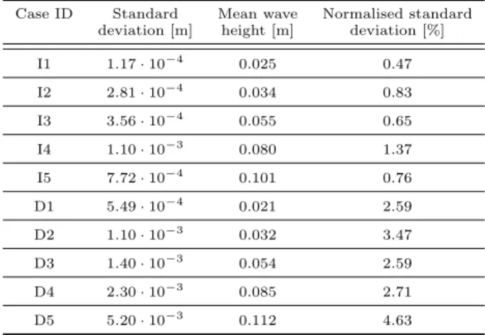
For a quantitative analysis, the standard deviation values, listed in Table 3, show values ranging from 1.17·10⁻⁴m to 5.2·10⁻³m, with a general trend towards larger standard deviations for the shorter period waves, D1 – D5. Normalisation by the mean wave height results in relative standard deviations between 0.36%

and 4.63%. According to [62], the typical accuracy for resistive wave gauges, as used for this experimental study, is±0.5mm. Thus, the standard deviation, for most of the considered regular waves, falls within the range of accuracy achievable with the measurement equipment.

4.2.2. Comparison to wave theory

Figures 7 (a) and (b) include the FSE described by 2^nd order Stokes wave theory. Qualitatively, a relatively close match between the theoretical and experimental data can be observed. For a quantitative analysis, the normalised Mean Absolute Percentage Error (nMAPE), between the experimental and theoretical phase-averaged FSE, is considered.

The nMAPE, for signals ofnsample points, is defined as follows:

nMAPE = 100%

n

X

i=1

|ηth(n)−η¯exp(n)

max(η_th) |. (9)

(17)

Table 3: Phase-averaged wave height and standard deviation at WP3

Case ID Standard Mean wave Normalised standard deviation [m] height [m] deviation [%]

I1 1.17·10⁻⁴ 0.025 0.47

I2 2.81·10⁻⁴ 0.034 0.83

I3 3.56·10⁻⁴ 0.055 0.65

I4 1.10·10⁻³ 0.080 1.37

I5 7.72·10⁻⁴ 0.101 0.76

D1 5.49·10⁻⁴ 0.021 2.59

D2 1.10·10⁻³ 0.032 3.47

D3 1.40·10⁻³ 0.054 2.59

D4 2.30·10⁻³ 0.085 2.71

D5 5.20·10⁻³ 0.112 4.63

In Equation (9),η_thdenotes the theoretical FSE, and ¯η_expthe mean experimental FSE from phase-averaging. The nMAPE is normalised by the maximum elevation of the considered wave. The results of the nMAPE, for waves I1–I5 and D1–D5, are plotted on the Le M´ehaut´e diagram in Figure 8. Overall, relatively small nMAPE values, between 0.3% and 5%, are found. A trend towards better agreement with wave theory can be noted for the short-period, deep water waves D1–D5. Furthermore, within the two groups of waves, a trend towards relatively larger nMAPE values, for the steeper waves, can be observed.

nMAPE

Figure 8: MAPE between experimental and theoretical elevations.

(18)

4.3. Velocity measurements

In this section, the water velocities beneath wave crests and troughs are analysed, comparing the PIV measurements against the theoretical results. Since the vertical velocity is zero directly beneath the crests and troughs, the analysis considers the horizontal water velocity component only. The zero vertical velocity characteristic is exploited to define the time instance of a wave crest or trough in the measured PIV data. In an iterative process, the vertical velocities at the available time instances from the PIV data set are analysed, and the time instance with vertical velocities closest to zero are defined as crest and trough events. Thus, the time instance of the crests and troughs are identified to within±0.023s. For the comparison with wave theory, the experimental results are averaged over 4 crests and troughs. The theoretical velocity values are computed based on Stokes 2^nd order wave theory, either employing both linear extrapolation and Wheeler stretching.

4.3.1. Velocity field data

The ability of PIV to generate velocity field data, spanning a defined interrogation window, provides a useful means to visualise the wave kinematics.

For example, Paprota [63] demonstrates the application of PIV to measuring the kinematics of a standing wave near a fully reflective wall and provides a qualitative analysis of the measured velocity fields (although no comparison to theory is presented). For the present study, the visualisation of the horizontal velocity fields, beneath the crests and the troughs, is shown in Figures 9 and 10, for case I1 (the least steep) and case D5 (the most steep), respectively. In these figures, the theoretical horizontal velocity fields, calculated using the extrapolation technique, are also provided for comparison, in addition to the the relative error, e, between the theoretical,uth and average experimental, ¯uexp, velocity values:

e(x, z) = u(x, z)_th−¯u(x, z)_exp u(x, z)th

·100%. (10) Qualitatively, the kinematics for the steeper wave, D5, appear to agree quite well with theory, whereas the kinematics for case I1 do not seem to match as closely with the theoretical results. Examining the quantitative comparison, provided by the relative error, the measured kinematics are generally within

±5−15% of the theoretical values, except for beneath the wave trough for I1, where the relative error is in the range of -25 to -35%.

(19)

-0.07 -0.065 -0.06 -0.055 -0.05 -0.045 -0.04

-30 -20 -10 0 10 20 30

-30 -20 -10 0 10 20 30 Error

e [%]

PIV

Horizontal veloticy[m/s]

Theory

Horizontal veloticy[m/s]

0.035 0.04 0.045 0.05 0.055 0.06

(a) Crest

(b) Trough Theory

Horizontal veloticy [m/s]

PIV

Error

e [%]

-0.07 -0.065 -0.06 -0.055 -0.05 -0.045 -0.04

Figure 9: Contour plots of the horizontal velocity under crests and troughs for case I1

(a) Crest

(b) Trough Theory

PIV

Error

e [%]

Error

e [%]

Vertical coordinate[mm]

PIV

Theory

-30 -20 -10 0 10 20 30 -30 -20 -10 0 10 20 30

Figure 10: Contour plots of the horizontal velocity under crests and troughs for case D5

4.3.2. Velocity profile

While the velocity field data provides an insightful visualisation, the reduced dimensionality of the velocity profile allows multiple attributes to be viewed si- multaneously. For example, the experimental data in Figure 11, shows the mean value and the 95% confidence interval (based on measurements of 4 wave periods), and is compared against theoretical values from both the linear extrapolation and Wheeler stretching methods. A qualitative analysis of the results

(20)

from the longer period waves, I1 and I5 in Figures 11 (a) and (b), reveals a consistent under–prediction of the theoretical velocity profile (for both extrapolation and Wheeler stretching) compared to the measured velocity profile. For the shorter period waves, D1 and D5 in Figures 11 (c) and (d), the experimental data is seen to agree well with the theoretical values, and also shows much smaller confidence intervals than for the longer period waves.

I

I5

Figure 11: Experimental and theoretical horizontal velocity profiles under the crests and troughs for cases I1 (a), I5 (b), D1 (c), and D5 (d) (see continuation of the figure below).

(21)

D

d D5

Cont. Figure 11: Experimental and theoretical horizontal velocity profiles under the crests and troughs for cases I1 (a), I5 (b), D1 (c), and D5 (d)

For a quantitative comparison of the measured velocity profiles versus theory, for all the 10 wave cases, two different metrics are used:

1. The relative error, as defined in Equation 10, for each sample point along the velocity profile atx= 0, compared to both the extrapolation technique and Wheeler stretching, as shown in Figure 12.

2. The nMAPE, as defined in Equation 9, giving a single mean value for the error along the the velocity profile at x = 0, compared to both the extrapolation technique and Wheeler stretching, as shown in Figures 13.

(22)

I I

I

e (f) D1

(g) D2 (h) D3

(i) D4 (j) D5

Figure 12: Relative deviation between experimental and theoretical horizontal velocity profiles under crests and troughs

Figures 12 (a)–(e) and (f)–(j), show the relative error for waves I1–I5 and D1–D5, respectively. For waves I1–I5, a larger error can generally be observed for the troughs (approx. 30%) compared to crests (10-20%). For waves D1–D5, more consistency between wave crests and trough is observed for relative error, and with generally smaller values (approx 10%). Furthermore, while the errors

(23)

calculated for waves I1–I5 indicate consistent under–prediction of the velocities, the errors for waves D1–D5 indicate both over– and under–prediction. Regard- ing the difference between the extrapolation technique and Wheeler stretching, neither approach delivers consistently better results. While, for some cases, the extrapolation technique results in smaller errors, for other cases Wheeler stretching results in better agreement with the experimental data.

Figure 13: nMAPE between PIV data and theoretical velocity profiles under wave crests and troughs using the extrapolation technique and Wheeler stretching

Considering the nMAPE values in Figures 13, for the longer period waves, I1–I5, a clear trend towards larger error values beneath the wave troughs (> 20%), compared to wave crests (15%), is visible. Interestingly, while the extrapolation technique shows larger nMAPE values underneath the trough, compared to Wheeler stretching, this trend is reversed underneath wave crests.

For the shorter period waves, D1–D5, overall consistent nMAPE values of<15%

are calculated underneath wave crests and troughs, with no significant dependency of the nMAPE on the use of either the extrapolation technique or Wheeler stretching.

4.4. Discussion

In consideration of the objectives; to provide a quantitative assessment of the ability of Stokes wave theory to describe the wave kinematics in practical wave tank testing situations, in which the finite length of the tank has a non-negligible effect, the following observations can be made.

The results show that the reflection coefficient varies for different wavelengths (Table 2). The installed beach has a fixed length, which appears to be more efficient for the wavelength of cases D1–D5, with larger reflection coefficients presenting for the longer waves, I1–I5. Furthermore, a dependency on

(24)

the wave height can be observed, where the reflection coefficient increases with increasing wave height. Overall, the achieved reflection coefficients (7% – 19%) fall within the common range of experimental test facilities [64].

Considering the FSE, Figure 8 shows that the error between the measured and theoretical values is generally larger for the cases with larger reflection coefficients (however case I1 is an outlier to this trend). An unexpected result, seen in Table 3, is that the standard deviation does not show proportionality to the determined reflection coefficients. In fact, larger standard deviations are calculated for waves D1–D5, while these waves show the smaller reflection coefficients than waves I1–I5.

For the wave kinematics, comparison of the measured velocity profiles against theory reveals that the error depends more on the wavelength than it does on the reflection coefficient. For a given wavelength, larger reflection coefficients generally lead to larger errors. However, all of the longer period waves, I1–I5, have significantly larger errors than all of the short period waves, D1–D5, even though D5 has a larger reflection coefficient than I1 and I2. A hypothesis to explain this observation is that the phase of the reflected wave, at the point of interest, is also as important as the reflection coefficient.

In this study, the distance from the measurement location (WP3) to the end of the tank and back is 25.49m. For the longer period waves, I1–I5, this distance relates to 7.94 wavelengths, meaning the reflected wave is approximately 180 degrees out of phase with the incident wave (since there is a 180 degrees phase shift at the reflection boundary). Therefore, at the measured crests and troughs of the incident waves, the reflected waves are approximately troughs and crests, thus will subtract from the measured wave height but add to the measured horizontal velocity (since the reflected wave is travelling in the opposite direction). Given that the theoretical velocity profiles are derived from the measured wave heights, the 180 degrees phase shift effectively doubles the influence of the reflective wave on the error in the velocity profile. For the short period waves, D1–D5, the distance from the measurement location to the end of the tank and back is 18.74 wavelengths, meaning the reflected wave is approximately 90 degrees out of phase with the incident wave. In this case, at the measured crests and troughs of the incident waves, the reflected waves are approximately zero-crossings, thus have negligible effect on the measured wave height and horizontal velocities.

5. Conclusions

The ability of Stokes wave theory to represent the wave kinematics in a short, physical wave flume is assessed based on a quantitative analysis of the measured FSE and velocity profile beneath wave crests and troughs, as well as the specific reflection coefficient for each different wave series. A set of ten regular wave series are investigated, spanning two different wavelengths and five amplitudes for each wavelength. The reflection coefficient is found to be depen- dent on the wavelength and amplitude, being larger on average for the longer period waves and also increasing with the wave amplitude, ranging from 7.3%

(25)

to 18.5%. Comparison of the measured FSE time series against theory shows a dependency on the reflection coefficient, with the error generally increasing for the wave series with larger reflection coefficients, ranging from 0.3% to 5%.

However, when comparing the measured velocity profiles against theory, the error is seen to not only depend on the reflection coefficient value, but also on the relative phase of the reflected wave, with respect to the incident wave, at the measurement location. Therefore, when conducting wave tank experiments in which reflections are present, in order to determine the wave kinematics from the FSE measurement using wave theory, it is not only necessary to the quan- tify the reflection coefficient value for each individual wave, but also the relative phase of the reflected wave at the point of interest.

Acknowledgment

This paper is based upon work supported by Science Foundation Ireland under Grant No. 13/IA/1886. Edward Ransley is funded by the Engineer- ing and Physical Sciences Research Council (EPSRC) in the United Kingdom (EP/M022382/1) through the Collaborative Computational Project in Wave Structure Interaction (CCP-WSI). The experimental test campaign was also funded by CCP-WSI and the test facility was provided by the COAST Labo- ratory, University of Plymouth. Josh Davidson is supported by the Higher Ed- ucation Excellence Program of the Ministry of Human Capacities in the frame of Water science & Disaster Prevention research area of Budapest University of Technology and Economics (BME FIKP-V´IZ).

References

[1] S. Barstow, G. Mørk, D. Mollison, J. Cruz, The Wave Energy Resource, Springer Berlin Heidelberg, Berlin, Heidelberg, 2008, pp. 93–132.

[2] O. Yagci, V. O. Kirca, L. Acanal, Wave attenuation and flow kinematics of an inclined thin plate acting as an alternative coastal protection structure, Applied Ocean Research 48 (2014) 214–226.

[3] N. Veritas, Environmental conditions and environmental loads, Det Norske Veritas, 2000.

[4] O. T. Gudmestad, Measured and predicted deep water wave kinematics in regular and irregular seas, Marine Structures 6 (1) (1993) 1–73.

[5] A. Natarajan, Influence of second-order random wave kinematics on the design loads of offshore wind turbine support structures, Renewable energy 68 (2014) 829–841.

[6] K. Tanizawa, S. Naito, A study on parametric roll motions by fully nonlinear numerical wave tank, in: Proceedings of the 7th International Offshore and Polar Engineering Conference, Honolulu, HI, USA, 1997.

(26)

[7] C. H. Kim, A. H. Clement, K. Tanizawa, Recent research and development of numerical wave tanks-a review, International Journal of Offshore and Polar Engineering 9 (1999).

[8] J. W. Kim, H. Jang, A. Baquet, J. O’Sullivan, S. Lee, B. Kim, H. Jasak, Technical and economic readiness review of CFD-based numerical wave basin for offshore floater design, in: Proceedings of the Offshore Technology Conference, Houston, TX, USA, 2016.

[9] C. Windt, J. Davidson, J. V. Ringwood, High-fidelity numerical modelling of ocean wave energy systems: A review of computational fluid dynamics- based numerical wave tanks, Renewable and Sustainable Energy Reviews 93 (2018) 610–630.

[10] J. Davidson, R. Costello, Efficient nonlinear hydrodynamic models for wave energy converter design—a scoping study, Journal of Marine Science and Engineering 8 (1) (2020) 35.

[11] A. Miquel, A. Kamath, M. Alagan Chella, R. Archetti, H. Bihs, Analysis of different methods for wave generation and absorption in a CFD-based numerical wave tank, Journal of Marine Science and Engineering 6 (2) (2018) 73.

[12] C. Windt, J. Davidson, P. Schmitt, J. V. Ringwood, On the assessment of numerical wave makers in CFD simulations, Journal of Marine Science and Engineering 7 (2) (2019) 47.

[13] I. R. Young, Encyclopedia of Maritine and Offshore Engieering, John Wiley and Sons, 2017, Ch. Regular, Irregular Waves and the Wave Spectrum, pp.

1–10. arXiv:https://onlinelibrary.wiley.com/doi/pdf/10.1002/

9781118476406.emoe078,doi:10.1002/9781118476406.emoe078.

URL https://onlinelibrary.wiley.com/doi/abs/10.1002/

9781118476406.emoe078

[14] M. J. Tucker, E. G. Pitt, Waves in ocean engineering, no. Volume 5, Else- vier, 2001.

[15] G. G. Stokes, On the theory of oscillatory waves, Transactions of the Cam- bridge Philosophical Society (1880).

[16] D. J. Korteweg, G. De Vries, XLI. On the change of form of long waves advancing in a rectangular canal, and on a new type of long stationary waves, The London, Edinburgh, and Dublin Philosophical Magazine and Journal of Science 39 (240) (1895) 422–443.

[17] M. Rienecker, J. Fenton, A Fourier approximation method for steady water waves, Journal of fluid mechanics 104 (1981) 119–137.

(27)

[18] R. J. Sobey, P. Goodwin, R. J. Thieke, R. J. Westberg Jr, Application of Stokes, Cnoidal, and Fourier wave theories, Journal of waterway, port, coastal, and ocean engineering 113 (6) (1987) 565–587.

[19] R. J. Sobey, Wave theory predictions of crest kinematics, in: Water wave kinematics, Springer, 1990, pp. 215–231.

[20] J. Zhang, R. E. Randall, C. A. Spell, Component wave interactions and irregular wave kinematics, Journal of waterway, port, coastal, and ocean engineering 118 (4) (1992) 401–416.

[21] H.-J. Jo, S.-J. Lee, J.-E. Choi, A study of flow structure of bichromatic waves through piv analysis, International Journal of Ocean System Engi- neering 2 (1) (2012) 8–15.

[22] R. E. Randall, J. Zhang, J. Longridge, Laser doppler anemometer measurements of irregular water wave kinematics, Ocean engineering 20 (6) (1993) 541–554.

[23] C. Spell, J. Zhang, R. E. Randall, Hybrid wave model for unidirectional irregular waves—part ii. comparison with laboratory measurements, Applied Ocean Research 18 (2-3) (1996) 93–110.

[24] J. Longridge, R. Randall, J. Zhang, Comparison of experimental irregular water wave elevation and kinematic data with new hybrid wave model predictions, Ocean engineering 23 (4) (1996) 277–307.

[25] H.-j. Choi, D. T. Cox, M. Kim, S. Ryu, Laboratory investigation of nonlinear irregular wave kinematics, in: Ocean Wave Measurement and Analysis (2001), 2002, pp. 1685–1694.

[26] A. Jensen, D. Clamond, M. Huseby, J. Grue, On local and convective accelerations in steep wave events, Ocean engineering 34 (3-4) (2007) 426–435.

[27] D. G. Dommermuth, D. K. Yue, W. Lin, R. Rapp, E. Chan, W. Melville, Deep-water plunging breakers: a comparison between potential theory and experiments, Journal of Fluid Mechanics 189 (1988) 423–442.

[28] C. Kim, R. Randall, M. Krafft, S. Boo, et al., Experimental study of kinematics of large transient wave in 2-d wave tank, in: offshore technology conference, Offshore Technology Conference, 1990.

[29] C. H. Kim, R. E. Randall, S. Y. Boo, M. J. Krafft, Kinematics of 2-D transient water waves using laser Doppler anemometry, Journal of waterway, port, coastal, and ocean engineering 118 (2) (1992) 147–165.

[30] J. Grue, D. Clamond, M. Huseby, A. Jensen, Kinematics of extreme waves in deep water, Applied Ocean Research 25 (6) (2003) 355–366.

(28)

[31] G. F. Clauss, F. Stempinski, M. Klein, Experimental and numerical analysis of steep wave groups, in: 12th International Congress of the International Maritime Association of the Mediterreanean, 2007.

[32] K. H. Jung, H.-j. Choi, S. B. Suh, H. J. Jo, Rogue wave kinematics in 2-d wave tank, in: INTELEC 2009-31st International Telecommunications Energy Conference, IEEE, 2009, pp. 1–8.

[33] H. Choi, S. Lee, H. Jo, G. Lee, K. Jung, Comparison study of experiments and predictions of wave kinematics for rogue wave, Brodogradnja 69 (1) (2018) 15 – 38.

[34] A. J. Martin, Laboratory simulation and numerical modelling of the kinematics of oceanic internal waves, Ph.D. thesis, University of Edinburgh (1997).

[35] M. Umeyama, H. Shinomiya, Particle image velocimetry measurements for stokes progressive internal waves, Geophysical Research Letters 36 (6) (2009).

[36] M. Umeyama, S. Matsuki, Measurements of velocity and trajectory of water particle for internal waves in two density layers, Geophysical research letters 38 (3) (2011).

[37] M. Umeyama, Eulerian–lagrangian analysis for particle velocities and trajectories in a pure wave motion using particle image velocimetry, Philo- sophical Transactions of the Royal Society A: Mathematical, Physical and Engineering Sciences 370 (1964) (2012) 1687–1702.

[38] J. Grue, J. Kolaas, Experimental particle paths and drift velocity in steep waves at finite water depth, Journal of Fluid Mechanics 810 (2017).

[39] J. Grue, J. Kolaas, On the lagrangian period in steep periodic waves, Water Waves 2 (1) (2020) 15–30.

[40] M. Paprota, W. Sulisz, A. Reda, Experimental study of wave-induced mass transport, Journal of Hydraulic Research 54 (4) (2016) 423–434.

[41] T. Van Den Bremer, C. Whittaker, R. Calvert, A. Raby, P. Taylor, Experi- mental study of particle trajectories below deep-water surface gravity wave groups, Journal of Fluid Mechanics 879 (2019) 168–186.

[42] Z. Zhang, LDA application methods: laser Doppler anemometry for fluid dynamics, Springer Science & Business Media, 2010.

[43] C. Swan, Wave kinematics within the crest to trough region, in: Environ- mental Forces on Offshore Structures and Their Predictions: Proceedings of an international conference, Society of Underwater Technology, 1990.

(29)

[44] J. Zhang, R. Randall, C. Spell, et al., On wave kinematics approximate methods, in: 23rd Annual Offshore Technology Conference, Houston, TX, USA, Offshore Technology Conference, 1991.

[45] F. Hering, C. Leue, D. Wierzimok, B. J¨ahne, Particle tracking velocimetry beneath water waves. part II: Water waves, Experiments in fluids 24 (1) (1998) 10–16.

[46] J. Grue, P.-F. Liu, G. Pedersen, PIV and water waves, Advances in Coastal and Ocean Engineering, Vol. 9, World Scientific, 2004.

[47] H.-J. Choi, Kinematics measurements of regular, irregular, and rogue waves by piv/ldv, Ph.D. thesis, Texas A&M University (2007).

[48] H. J. Choi, K. H. Jung, S. Suh, H. J. Jo, H. S. Choi, Experimental study on nonlinearity characteristics near the free surface in the regular wave condition, Journal of Ocean Engineering and Technology 24 (1) (2010) 1–

9.

[49] A. Jensen, J. K. Sveen, J. Grue, J.-B. Richon, C. Gray, Accelerations in water waves by extended particle image velocimetry, Experiments in fluids 30 (5) (2001) 500–510.

[50] T. Kristiansen, R. Baarholm, G. J. Rortveit, E. W. Hansen, C. T. Stans- berg, Kinematics in a diffracted wave field: particle image velocimetry (PIV) and numerical models, in: ASME 2005 24th International Conference on Offshore Mechanics and Arctic Engineering, Halkidiki, Greece, Ameri- can Society of Mechanical Engineers Digital Collection, 2005, pp. 827–835.

[51] M. Umeyama, Coupled PIV and PTV measurements of particle velocities and trajectories for surface waves following a steady current, Journal of Waterway, Port, Coastal, and Ocean Engineering 137 (2) (2010) 85–94.

[52] J. Grue, J. Kolaas, A. Jensen, Velocity fields in breaking-limited waves on finite depth, European Journal of Mechanics-B/Fluids 47 (2014) 97–107.

[53] J. Fenton, The numerical solution of steady water wave problems, Com- puters & Geosciences 14 (3) (1988) 357–368.

[54] D. Vargas, R. Jayaratne, E. Mendoza, R. Silva, On the estimation of the surface elevation of regular and irregular waves using the velocity field of bubbles, Journal of Marine Science and Engineering 8 (2) (2020) 88.

[55] T. B. Johannessen, Calculations of kinematics underneath measured time histories of steep water waves, Applied Ocean Research 32 (4) (2010) 391–

403.

[56] Edinburgh Design, Edinburgh Design wave gauges product website,http:

//www4.edesign.co.uk/product/wavegauges/, last accessed 2020-07-21 (2020).

(30)

[57] J. K. Sveen, E. A. Cowen, Quantitative imaging techniques and their application to wavy flows, in: PIV and water waves, World Scientific, 2004, pp. 1–49.

[58] B. Le M´ehaut´e, An introduction to hydrodynamics and water waves, Springer Science & Business Media, 1969.

[59] R. Dean, Water wave kinetics: State of the art and future research needs, in: Water Wave Kinematics, Springer, 1990, pp. 743–756.

[60] J. Wheeler, Method for calculating forces produced by irregular waves, Journal of petroleum technology 22 (3) (1970) 359–367.

[61] E. Mansard, E. Funke, The measurement of incident and reflected spectra using a least squares method, in: Coastal Engineering 1980, 1980, pp. 154–

172.

[62] S. Masterton, C. Swan, On the accurate and efficient calibration of a 3D wave basin, Ocean Engineering 35 (8) (2008) 763 – 773.

[63] M. Paprota, Particle image velocimetry measurements of standing wave kinematics in vicinity of a rigid vertical wall, Instruments and Experimental Techniques 62 (2) (2019) 277–282.

[64] J. Cruz, Ocean wave energy: current status and future prespectives, Springer Science & Business Media, 2007.