INTRODUCTION
THE MAXIMUM A
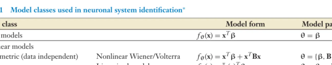
The Model Class
Each model class implies strong assumptions about the functional properties that a neuron may exhibit. To get a good estimate of the map function, it is important to choose a model class that can provide a good description of the neuron. The model class first used to describe nonlinear sensory neurons is the Wiener or Volterra series (Aertsen & Johannesma.
In this case, the linear model is considered to be the first-order term of the expansion of the mapping function into a Wiener or Volterra series. It is usually not feasible to estimate the terms of the full Wiener/Volterra model beyond second order because the amount of data needed to estimate each higher-order term depends exponentially on the order of the model (Victor 2005). Since the fixed-order Wiener/Volterra model is parametric, it can be considered as a linearized model whose linearizing transformation is described by nonlinear terms of the series expansion (David & . Gallant 2005).
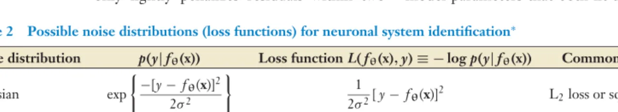
The Noise Distribution
Many linearized models implement the initial nonlinearity in a preprocessing step; in these cases the subsequent linear-nonlinear phases are placed separately (Aertsen & Johannesma 1981b, Eggermont 1993).
The Prior (Regularizer)
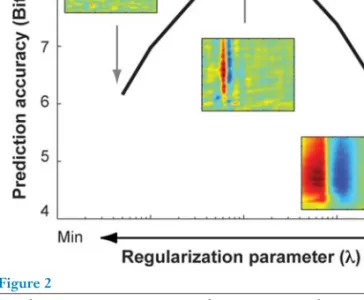
In practice, the relative influence between the loss function and the regulator must be tuned by cross-validation to achieve an accurate estimate of the mapping function (Figure 2) (Section 3.3). These algorithms implicitly assume that all model parameter values are equally likely (flat prior). Natural stimuli contain strong correlations that can introduce noise into the mapping function estimates.
Low values of the adjustment parameter do not remove much high-frequency noise, so the predictions are poor. The associated regularizer (column 4) is obtained by taking the negative log of the prior.σ2θ is the variance of each model parameter, which is the same for all model parameters in the spherical parameter.σ2θ. Computationally, the pre-stimulus subspace adjuster will impose infinite penalties on the target MAP whenever an associated small eigenvalue parameter is nonzero.
COMPUTING THE
Properties of the MAP
The spherical Gaussian parameters are independent with equal variance A=σ2θI σ−2θθ22=σ−2θ θk2 The former independence parameters are completely independent A=diag(σ2θ . k). The prior smooth parameters vary smoothly over the stimulus dimensions A=D−2 δ−1θTD2θ=δ−1Dθ22 The stimulus subspace parameters lie within a principal component subspace of the stimulus A=QDλQT. The pre-stimulus subspace applies a threshold operation to force the parameter values to zero for those principal components with eigenvalues less than λ.
The stimulus subspace prior can be used to attenuate high-frequency noise when using natural stimuli to estimate the mapping functions. This prerequisite requires specifying a regularization parameter for the noise threshold, which is usually set via cross-validation (David et al. 2004, Theunissen et al. 2001) (Figure 2 and Section 3.3). Loss function (noise distribution) RegularizerAssumptionsandpriorparametersObjectivefunction#afmodelparameters#affreeparameters Spike-triggeredaverageLinearL2loss(Gaussian)ConstantAllvaluesfairlyprobable:fladprior A−1=0Nolocalminimaandsmoothed+10lossisLensqual. lylikely:flatprior A−1=0Nolocalminimaand smoothed+10 RidgeregressioncLinearL2tab(Gaussian)σ −2 ββ2 2Independentwithequalvariance: Gaussian A=σ2 θINlocal minimumand smooth.
To simplify the calculation, most SI studies in neurophysiology use algorithms that have a smooth MAP objective function without local minima. The simplest of these consists of a linear model class, a Gaussian noise distribution and a Gaussian prior (LGG family, shaded entries in Table 4). The MAP measure of any algorithm in the LGG family can be minimized analytically.
Here λ = σ2 is the noise variance (Table 2), and A is the covariance matrix of the Gaussian prior. When the stimulus is white noise, there are no correlations between stimulus channels and the stimulus autocovariance, XTX, is trivially the identity matrix (Victor 2005).
Number of Model
Number of Free Parameters
EXPERIMENTAL
- Stimulus Selection
- Behavioral Control
- Visualization and
- Prediction and Validation
For this reason, most studies that have used white noise to estimate second-order Wiener/Volterra models have been conducted in simple organisms or in peripheral sensory systems (Brenner et al. 2000, Pece et al. 1990). . High-contrast noise is often used in combination with the m-sequence method to maximize stimulus sampling efficiency (Cottaris & De Valois 1998, Reid et al. 1997, Sutter 1987). This increases the local contrast in the stimulus and generally produces more robust responses (DeAngelis et al.
The parameters defining these stimuli can be a linear function of the stimulus ( Yu & de Sa 2004 ) or a non-linear function such as spectral power ( Aertsen & Johannesma 1981b ) or orientation ( Ringach et al. 1997b ). Parametric moving dot noise has also been used in motion-sensitive area MT (Borghuis et al. 2003, Cook & Maunsell 2004). However, mapping functions estimated using these subsets do not necessarily generalize to the entire space of natural stimuli (David et al. 2004).
There is increasing evidence that the stimulus-response mapping function of sensory neurons can be modified by top-down effects such as attention (David et al. 2002, Fritz et al. 2003) and learning (Polley et al. With the assumption Because this task induces a consistent cognitive state, the mapping function can then be estimated directly without modeling top-down effects (David et al. 2004).Second-order Wiener/Volterra models can typically be visualized by mapping the relevant stimulus subspace. (Brenner et al. 2000, Rust et al. 2005, Touryan et al. 2002).
This subspace can be extracted from the model parameters by dimensionality reduction (e.g. singular value decomposition), and the relevant stimulus subspace can be directly visualized (Figure 3) (Lau et al. 2002, Prenger et al.). 2004). This is a particular hazard when comparing map functions estimated using different stimuli, different data sets, or different regularization schemes (David et al. 2004, Sharpee et al. 2004). The correlation coefficient provides an intuitive measure of predictive power: the squared correlation coefficient represents the fraction of response variance explained by the model (David & Gallant 2005, Machens et al. 2004, Sahani & Linden 2003b).
Other measures of predictive power have been proposed that may be more suitable for neuronal spike data [e.g., coherence (Hsu et al. 2004), mutual information (Sharpie et al. 2004)].
APPLICATIONS
- Tuning Properties
- Nonlinear Response
- Functional Anatomy
- Natural Stimuli
- Cognitive Factors
- Optimal Stimuli
- Predictive Power
Analysis of mapping functions in the LGN suggests that the population of retinal ganglion cells is optimized for conveying information about natural scenes (Dan et al. 1996). Similarly, the neuronal tuning in the songbird auditory thalamus appears to be optimized for representing song (Woolley et al. 2005). Second-order Wiener/Volterra models (Citron & Emerson 1983, Eggermont 1993, Mancini et al. 1990) have been extremely useful in characterizing neurons in many sensory systems.
These findings are broadly consistent with the predictions of the kinetic energy model (Emerson et al. 1992, Gaska et al. 1994). Therefore, more flexible nonparametric models have been used to investigate effects such as nonlinear spatial pooling (Prenger et al. 2005, Wu & Gallant 2004). Mapping functions have also been estimated for connected pairs of neurons in the auditory thalamus and cortex (Miller et al. 2001).
Natural stimuli contain rich combinations of features that can drive these context-dependent responses in ways that cannot be predicted with simple synthetic stimuli (David et al. 2004). Furthermore, V1 neurons will adapt to the statistics of natural stimuli to increase information transfer (Sharpee et al. 2006). These processes change the way sensory information is routed and packaged in successive stages of representation (Olshausen et al. 1993).
To investigate cognitive factors from the SI perspective, it is useful to view them as additional input channels (David et al. 2002). If these are separable, attention merely modulates the response rate (Luck et al. 1997) or gain (McAdams & Maunsell 1999, Reynolds & Chelazzi 2004) of a neuron. In contrast, studies in areas V4 (David et al. 2002) and A1 (Fritz et al. 2003) reported that attention can also modulate tuning properties.
Invariant tuning becomes even more common at more central stages of visual processing [e.g., inferior temporal cortex (Ito et al. 1995)].
FUTURE DIRECTIONS
Simple synthetic stimuli are experimentally appropriate, but the ultimate test of any model of sensory processing is how well it predicts neural responses to natural stimuli during natural sensory exploration (Carandini et al. 2005, David & Gallant 2005). These predictions are uniformly lower than those obtained for simple stimuli, reflecting the complexity of natural signals and the fact that such signals often elicit non-linear responses not seen with simpler stimuli (David et al. 2004, Theunissen et al. 2000, Woolley et al. 2005). No SI studies have assessed prediction during natural sensory exploration; this is a likely avenue for future research.
CONCLUSIONS
Efficient encoding of natural scenes in the lateral geniculate nucleus: experimental test of a computational theory.J. Direction-selective complex cells and the computation of motion energy in cat visual cortex.Vis. Visual cortex neurons of monkeys and cats: temporal dynamics of the spatial frequency response function.J.
Space-time spectra of complex cell filters in the macaque: a comparison of results obtained with pseudowhite noise and grating stimuli.Vis. The influence of contextual stimuli on the orientation selectivity of cells in the primary visual cortex of the cat.Fish. Representation of temporal features of complex sounds by the discharge patterns of neurons in the inferior colliculus of the owl.J.
Neuronal selectivities for complex object features in the ventral visual pathway of the macaque cerebral cortex.J. Receptive field properties of neurons in early visual cortex revealed by local spectral inverse correlation.J. Direction selectivity of excitation and inhibition in simple cells of the cat primary visual cortex. Neuron45:133–45.
Use of m-sequences in the analysis of visual neurons: properties of the linear receptive field. Height Receptor field structure of neurons in monkey primary visual cortex revealed by stimulation with natural picture sequences. J. Receptive field organization of simple cells in the primary visual cortex of ferrets during natural scene stimulation.
Stimulus-dependent auditory tuning leads to synchronous population coding of vocalizations in the songbird midbrain.J.