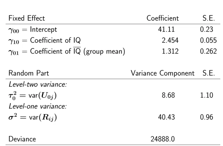
If the researcher is only interested in within-group effects, and is suspicious of the model for between-group differences, then F is more robust. The within-group regression coefficient is the regression coefficient within each group, which is assumed to be the same across the groups. The between-group regression coefficient is defined as the regression coefficient for the regression of the group means of Y on the group means of X.
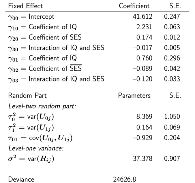
This is convenient because the difference between within-group and between-group coefficients can be tested by considering γ01. In the model with special effects for the group-centered variable x˜ij and the group mean. This is convenient because these coefficients are immediately given in the results, with their standard errors.
The random effects U0j are not statistical parameters and are therefore not estimated as part of the estimation routine. In statistical terminology, this is not called an 'estimate', but a 'prediction', the name for the construction of probable values for unobserved random variables.
The hierarchical linear model
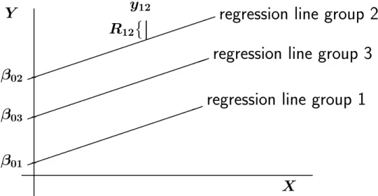
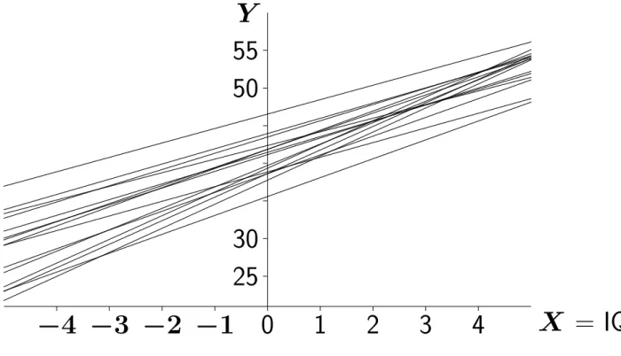
The group dependent coefficients (U0j, U1j) are assumed to be independent over j, with a bivariate normal distribution with expected values (0, 0) and covariance matrix defined by. We therefore have a linear model for the mean structure, and a parameterized covariance matrix within groups with independence between groups. Intercept variance and intercept-slope covariance depend on the position of the X = 0 value, because the intercept is defined by the X = 0 axis.
Testing
The simplest test for all parameters (fixed and random parts) is the variance (likelihood ratio) test that we can use. If these two models do not have the same fixed parts, the ML estimate should be used. Other tests have been developed for the parameters in the random part that are similar to the F-tests in ANOVA.
The interpretation is that if the observed between-group variance is less than expected under the null hypothesis. For example: test for a random slope in a model that also contains the random intercept, but no other random slopes: p = 1;.
Explained variance
The best way to define R2, the explained portion of the variance, is the proportional reduction of the total variance.
Heteroscedasticity
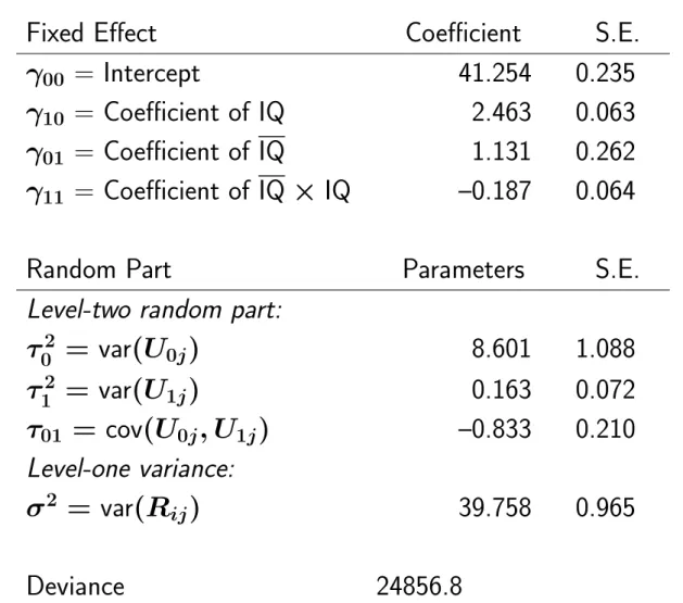
However, the following models show that the heteroscedasticity as a function of IQ is more important.
Assumptions of the Hierarchical Linear Model
Include the fixed effect of X¯h if it is significant, and continue to use a random effects model. There are often substantive interpretations of the difference between the effects within the group γ2 and the effects between the groups γ1. Test the fixed part of the level-1 model using OLS level-1 residuals, calculated separately per group.
In other words, the level 1 specification can be studied by dividing at the within-group level. comparable to a "fixed effects analysis"). The construction of the within-group OLS residuals implies that this only tests the level one specification. regardless of the correctness of the second-level specification. Mean level OLS residuals. bars ~ twice standard error of the mean) as a function of IQ.
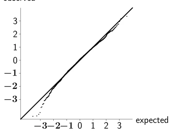
The deletion-standardized multivariate residual can be used to assess the fit of group j, but removes the effect of this group on the parameter estimates. j) meaning that group j is removed from the data for estimating this parameter.
Designing Multilevel Studies
Sandwich estimators
This way of calculating standard errors does not rely on a specific random effect specification, nor on normality of the residuals. Another problem is that the model is incompletely specified: the random part of the model is ignored. For the latter two questions, the degree of imbalance between the groups will be an issue.
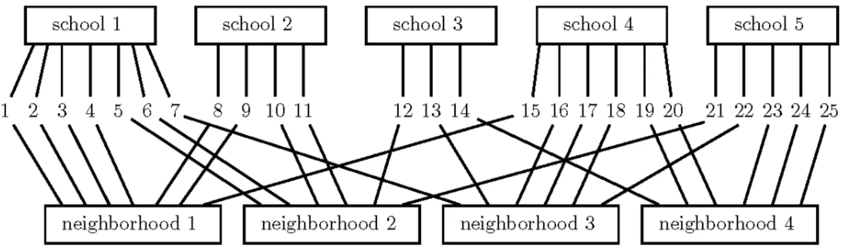
Imperfect Hierarchies
Correlation between exam grades of students who attended the same primary school but went to a different secondary school. Correlation between grades of students who attended the same high school but came from different primary schools. Correlation between grades of students who attended the same primary and secondary school.
Individuals are/have been members of several social units (such as several different high schools). Just a random factor at level two. compared to two or more factors in cross-classified models). Denote by Yi{j} an individual that can have multiple membership. Write the HLM with second-level residuals U0h weighted by wih.
Survey weights
If the model is specified correctly given all the design variables, ie. the residuals in the model are independent of the design variables, then the sample design can be ignored in the analysis. We argue for, whenever possible, aiming for a model-based analysis, where the analysis is based on the design variables. Grouping by design weights is important here because the assumption for a model-based analysis is that the model does not depend on the design weights.
Execute model-based and design-based elements within each Level 2 unit and compare results. Once again this is done in the hope of being able to opt for a model-based model. Design and model-based estimates for three ratios, for public schools in the South.
Estimates for a model of metacognitive competence, including urbanization, for five parts of the dataset: fixed effects. Estimates for a model of metacognitive competence, including urbanization, for five parts of the dataset: variance parameters. Design-based and model-based estimates for metacognitive competence model, full data set: fixed effects.
Design-based and model-based estimates of the model for metacognitive competence, the entire data set: variance parameters. Design-based and model-based evaluations of the model for metacognitive competence, public schools without outliers: fixed effects. Design-based and model-based evaluations of the model for metacognitive competence, public schools without outliers: variance parameters.
Design-Based and Model-Based Estimates of a Model for Metacognitive Competence, Non-Exit Public Schools, with More Extensive Controls: Fixed Effects. Design-based and model-based estimates of a model for metacognitive competence, non-dropout public schools, with more extensive controls: Variance parameters. For the student-level variables, the final model-based results are almost indistinguishable from the model-based results for the entire data set, accounting for urbanization.
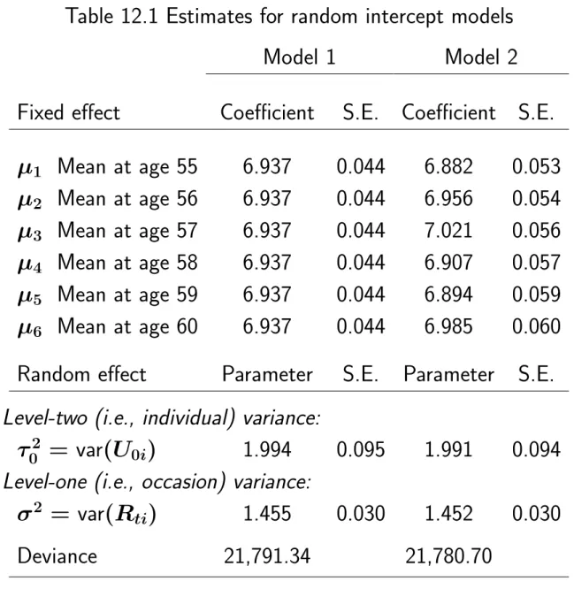
Longitudinal data
Note that these correlations are the same between all measurements of the same subject, whether they are for adjacent or far apart waves. Individual respondents are likely to vary not only in their mean value over time, but also in the rate of change and other aspects of time dependence. This is modeled by including random time slopes, and nonlinear time transformations.
Note that age is included non-linearly as a main effect (dummy variables) and linearly in interaction with year of birth. Since age ranges from 0 to 5 years, this represents greater variation in the rate of change than that explained by year of birth. A further option available for fixed occasion data. not in this way for variable opportunity data) is the fully multivariate model, which imposes no restrictions on the covariance matrix.
For the REML estimation method, this method reproduces the paired-samples t-test if data are complete. It follows that growth in this age range is quite nearly linear, with an average growth rate of 5.53 cm/y. The advantage of piecewise linear functions is that they are less globally sensitive to local changes in the function values.
The correlation matrix is given only for completeness, not because we can see much from it.
Discrete dependent variables
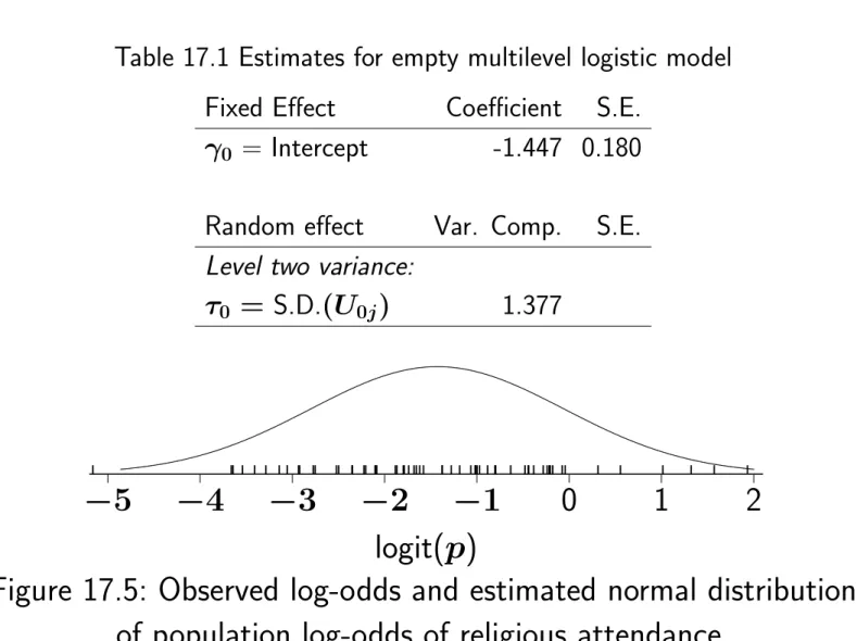
One of the most widely used transformations of probabilities is log odds, defined by. The logit function, graphs of which are shown here, is an increasing function defined for numbers between 0 and 1, and its range is from minus infinity to plus infinity. Estimated level-2 intercept variance can increase when level-1 variables are added, and always do so when these have no between-group variance.
The fact that the level 1 latent variance is fixed implies that the level 1 variance is explained by the new variable Xr+1. A measure of explained variance ('R2') for multilevel logistic regression can be based on this representation of the threshold as is. Number of memberships in voluntary organizations of individuals in 40 regions in the Netherlands (ESS data).