Divergence measures for comparing distributions and training generative models: Part 2
Arthur Gretton
Gatsby Computational Neuroscience Unit, University College London
DeepLearn, 2022
1/34
Training generative models
Have: One collection of samplesX from unknown distributionP.
Goal: generate samplesQ that look like P
LSUN bedroom samples P GeneratedQ, MMD GAN
Role of divergence D ( P ; Q ) ?
2/34
Outline
-divergences (f-divergences) and a variational lower bound (KL) Generalized energy-based models
“Like a GAN” but incorporatecritic into sample generation Perform better than usinggeneratoralone
Arbel, Zhou, G., Generalized Energy Based Models (ICLR 2021)
3/34
Divergences
4/34
Divergences
5/34
The Integral Probability Metrics
6/34
Maximum mean discrepancy
Ahelpful critic witness:
MMD(P;Q) = supkfkF1EPf(X) EQf(Y).
MMD=1.8
7/34
Maximum mean discrepancy
Ahelpful critic witness:
MMD(P;Q) = supkfkF1EPf(X) EQf(Y) MMD=1.1
7/34
The -divergences
8/34
The -divergences
Define the-divergence(f-divergence):
D(P;Q) = Z
p(z)
q(z)
q(z)dz whereis convex, lower-semicontinuous,(1) =0.
Example: (u) =ulog(u) gives KL divergence, DKL(P;Q) =Z log
p(z) q(z)
p(z)dz
=Z p(z) q(z)
log
p(z) q(z)
q(z)dz
9/34
The -divergences
Define the-divergence(f-divergence):
D(P;Q) = Z
p(z)
q(z)
q(z)dz whereis convex, lower-semicontinuous,(1) =0.
Example: (u) =ulog(u) gives KL divergence, DKL(P;Q) =Z log
p(z) q(z)
p(z)dz
=Z p(z) q(z)
log
p(z) q(z)
q(z)dz
9/34
Are -divergences good critics?
Simple example: disjoint support.
Goodfellow et al. (NeurIPS 2014), Arjovsky and Bottou [ICLR 2017]
DKL(P;Q) = 1 DJS(P;Q) = log2
10/34
Are -divergences good critics?
Simple example: disjoint support.
Goodfellow et al. (NeurIPS 2014), Arjovsky and Bottou [ICLR 2017]
DKL(P;Q) = 1 DJS(P;Q) = log2
10/34
-divergences in practice
Background: the conjugate (Fenchel) dual (v) = sup
u2Rfuv (u)g :
(v) is negative intercept of tangent towith slopev
11/34
-divergences in practice
Background: the conjugate (Fenchel) dual (v) = sup
u2Rfuv (u)g :
For a convex l.s.c. we have
(x) = (x) = sup
v2Rfxv (v)g
11/34
-divergences in practice
Background: the conjugate (Fenchel) dual (v) = sup
u2Rfuv (u)g :
For a convex l.s.c. we have
(x) = (x) = sup
v2Rfxv (v)g
KL divergence:
(x) =xlog(x) (v) = exp(v 1)
11/34
A variational lower bound
A lower-bound-divergence approximation:
D(P;Q) =Z q(z) p(z)
q(z)
dz
sup
f2HEPf(X) EQ(f(Y)) (restrict thefunction class)
(v)is dual of (x):
Bound tight when:
f(z) = @ p(z)
q(z) if ratio defined.
Nguyen, Wainwright, Jordan, IEEE Transactions on Information Theory (2010);
Nowozin, Cseke, Tomioka, NeurIPS (2016)
12/34
A variational lower bound
A lower-bound-divergence approximation:
D(P;Q) =Z q(z) p(z)
q(z)
dz
=Z q(z)sup
fz
p(z)
q(z)fz (fz)
| {z }
pq((zz))
sup
f2HEPf(X) EQ(f(Y)) (restrict thefunction class)
(v)is dual of (x):
Bound tight when:
f(z) = @ p(z)
q(z) if ratio defined.
Nguyen, Wainwright, Jordan, IEEE Transactions on Information Theory (2010);
Nowozin, Cseke, Tomioka, NeurIPS (2016)
12/34
A variational lower bound
A lower-bound-divergence approximation:
D(P;Q) =Z q(z) p(z)
q(z)
dz
=Z q(z) sup
fz
p(z)
q(z)fz (fz)
sup
f2HEPf(X) EQ(f(Y)) (restrict thefunction class)
(v)is dual of (x):
Bound tight when:
f(z) = @ p(z)
q(z) if ratio defined.
Nguyen, Wainwright, Jordan, IEEE Transactions on Information Theory (2010);
Nowozin, Cseke, Tomioka, NeurIPS (2016)
12/34
Case of the KL
DKL(P;Q) =Z log p(z)
q(z)
p(z)dz
Nguyen, Wainwright, Jordan, IEEE Transactions on Information Theory (2010);
Nowozin, Cseke, Tomioka, NeurIPS (2016)
13/34
Case of the KL
DKL(P;Q) =Z log p(z)
q(z)
p(z)dz sup
f2H EPf(X) +1 EQexp (| {zf(Y))}
( f(Y)+1)
Nguyen, Wainwright, Jordan, IEEE Transactions on Information Theory (2010);
Nowozin, Cseke, Tomioka, NeurIPS (2016)
13/34
Case of the KL
DKL(P;Q) =Z log p(z)
q(z)
p(z)dz sup
f2H EPf(X) +1 EQexp ( f(Y))
Bound tight when:
f(z) = logp(z) q(z) if ratio defined.
Nguyen, Wainwright, Jordan, IEEE Transactions on Information Theory (2010);
Nowozin, Cseke, Tomioka, NeurIPS (2016)
13/34
Case of the KL
DKL(P;Q) =Z log p(z)
q(z)
p(z)dz sup
f2H EPf(X) +1 EQexp ( f(Y)) sup
f2H
2 4 1
n Xn j=1
f(xi) 1 n
Xn i=1
exp( f(yi)) 3 5+1
xi i:i:d:P yi i:i:d:Q
Nguyen, Wainwright, Jordan, IEEE Transactions on Information Theory (2010);
Nowozin, Cseke, Tomioka, NeurIPS (2016)
13/34
Case of the KL
DKL(P;Q) =Z log p(z)
q(z)
p(z)dz sup
f2H EPf(X) +1 EQexp ( f(Y)) sup
f2H
2 4 1
n Xn j=1
f(xi) 1 n
Xn i=1
exp( f(yi)) 3 5+1
This is a KL
Approximate Lower-bound Estimator.
Nguyen, Wainwright, Jordan, IEEE Transactions on Information Theory (2010);
Nowozin, Cseke, Tomioka, NeurIPS (2016) 13/34
Case of the KL
DKL(P;Q) =Z log p(z)
q(z)
p(z)dz sup
f2H EPf(X) +1 EQexp ( f(Y)) sup
f2H
2 4 1
n Xn j=1
f(xi) 1 n
Xn i=1
exp( f(yi)) 3 5+1
This is a K A L E
Nguyen, Wainwright, Jordan, IEEE Transactions on Information Theory (2010);
Nowozin, Cseke, Tomioka, NeurIPS (2016) 13/34
Case of the KL
DKL(P;Q) =Z log p(z)
q(z)
p(z)dz sup
f2H EPf(X) +1 EQexp ( f(Y)) sup
f2H
2 4 1
n Xn j=1
f(xi) 1 n
Xn i=1
exp( f(yi)) 3 5+1
The KALE divergence
Nguyen, Wainwright, Jordan, IEEE Transactions on Information Theory (2010);
Nowozin, Cseke, Tomioka, NeurIPS (2016)
13/34
Empirical properties of KALE
KALE(P;Q;H) = sup
f2H EPf(X) EQexp ( f(Y)) +1 f = hw; (x)iH Han RKHS
kwk2H penalized:
KALE smoothie KALE(Q;P;H)=0.12
Glaser, Arbel, G. “KALE Flow: A Relaxed KL Gradient Flow for Probabilities with
Disjoint Support,” (NeurIPS, 2021, Section 2) 14/34
Empirical properties of KALE
KALE(P;Q;H) = sup
f2H EPf(X) EQexp ( f(Y)) +1 f = hw; (x)iH Han RKHS
kwk2H penalized:KALE smoothie
KALE(Q;P;H)=0.12
Glaser, Arbel, G. “KALE Flow: A Relaxed KL Gradient Flow for Probabilities with
Disjoint Support,” (NeurIPS, 2021, Section 2) 14/34
Empirical properties of KALE
KALE(P;Q;H) = sup
f2H EPf(X) EQexp ( f(Y)) +1 f = hw; (x)iH Han RKHS
kwk2H penalized:KALE smoothie KALE(Q;P;H)=0.18
KALE(Q;P;H)=0.12
Glaser, Arbel, G. “KALE Flow: A Relaxed KL Gradient Flow for Probabilities with
Disjoint Support,” (NeurIPS, 2021, Section 2) 14/34
Empirical properties of KALE
KALE(P;Q;H) = sup
f2H EPf(X) EQexp ( f(Y)) +1 f = hw; (x)iH Han RKHS
kwk2H penalized:KALE smoothie KALE(Q;P;H)=0.12
Glaser, Arbel, G. “KALE Flow: A Relaxed KL Gradient Flow for Probabilities with
Disjoint Support,” (NeurIPS, 2021, Section 2) 14/34
The KALE smoothie and “mode collapse”
Two Gaussians with same means, different variance
“Mode collapse”
Example thanks to M. Arbel and M. Rosca 15/34
Topological properties of KALE (1)
Key requirements onH andX: Compact domainX,
Hdense in the spaceC(X )of continuous functions on X wrtk k1. Iff 2Hthen f 2H and cf 2Hfor 0c Cmax.
Theorem: KALE(P;Q;H) 0 andKALE(P;Q;H) =0 iffP =Q.
Hdense inC(X )forX Rd when:
H=spanf(w>x +b) : [w;b] 2 g (u) = maxfu;0g; 2 N, and f : 0; 2 g = Rd+1.
Zhang, Liu, Zhou, Xu, and He. “On the Discrimination-Generalization Tradeoff in GANs”
(ICLR 2018, Corollary 2.4; Theorem B.1) Arbel, Liang, G. (ICLR 2021, Proposition 1)
16/34
Topological properties of KALE (2)
Additional requirement: all functions inH Lipschitz in their inputs with constantL
Theorem: KALE(P;Qn;H) !0 iffQn !P under the weak topology.
Partial proof idea:
KALE(P;Q;H) = Z fdP Z
exp( f)dQ+1
=Z f(x)dQ(x) f(x0)dP(x0) Z
(exp( f) +f 1)
| {z }
0
dQ
Z
f(x)dQ(x) f(x0)dP(x0) LW1(P;Q)
Liu, Bousquet, Chaudhuri. “Approximation and Convergence Properties of Generative Adversarial Learning” (NeurIPS 2017); Arbel, Liang, G. (ICLR 2021, Proposition 1)17/34
How to train your GAN
Generalized Energy-Based Model
18/34
Visual notation: GAN setting
19/34
Visual notation: GAN setting
generate
19/34
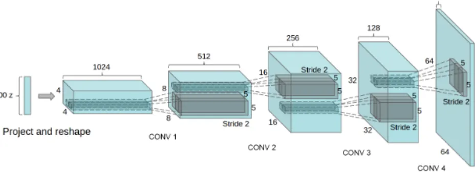
Reminder: the generator
Under review as a conference paper at ICLR 2016Figure 1: DCGAN generator used for LSUN scene modeling. A 100 dimensional uniform distribu- tionZis projected to a small spatial extent convolutional representation with many feature maps.
A series of four fractionally-strided convolutions (in some recent papers, these are wrongly called deconvolutions) then convert this high level representation into a64⇥64pixel image. Notably, no fully connected or pooling layers are used.
suggested value of 0.9 resulted in training oscillation and instability while reducing it to 0.5 helped stabilize training.
4.1 LSUN
As visual quality of samples from generative image models has improved, concerns of over-fitting and memorization of training samples have risen. To demonstrate how our model scales with more data and higher resolution generation, we train a model on the LSUN bedrooms dataset containing a little over 3 million training examples. Recent analysis has shown that there is a direct link be- tween how fast models learn and their generalization performance (Hardt et al., 2015). We show samples from one epoch of training (Fig.2), mimicking online learning, in addition to samples after convergence (Fig.3), as an opportunity to demonstrate that our model is not producing high quality samples via simply overfitting/memorizing training examples. No data augmentation was applied to the images.
4.1.1 DEDUPLICATION
To further decrease the likelihood of the generator memorizing input examples (Fig.2) we perform a simple image de-duplication process. We fit a 3072-128-3072 de-noising dropout regularized RELU autoencoder on 32x32 downsampled center-crops of training examples. The resulting code layer activations are then binarized via thresholding the ReLU activation which has been shown to be an effective information preserving technique (Srivastava et al., 2014) and provides a convenient form of semantic-hashing, allowing for linear time de-duplication . Visual inspection of hash collisions showed high precision with an estimated false positive rate of less than 1 in 100. Additionally, the technique detected and removed approximately 275,000 near duplicates, suggesting a high recall.
4.2 FACES
We scraped images containing human faces from random web image queries of peoples names. The people names were acquired from dbpedia, with a criterion that they were born in the modern era.
This dataset has 3M images from 10K people. We run an OpenCV face detector on these images, keeping the detections that are sufficiently high resolution, which gives us approximately 350,000 face boxes. We use these face boxes for training. No data augmentation was applied to the images.
4
Radford, Metz, Chintala, ICLR 2016
20/34
Energy function to improve generator: demo
Targetdistribution P
Example thanks to M. Arbel
21/34
Energy function to improve generator: demo
GAN (generator)Q,correct supportbut wrong mass
Example thanks to M. Arbel
21/34
Energy function to improve generator: demo
Log energy functionand Q
Key:
Orange: increase mass Blue: reduce mass
Example thanks to M. Arbel 21/34
Energy function to improve generator: demo
Targetdistribution P and GAN (generator) Q,wrong supportand wrong mass
Example thanks to M. Arbel
21/34
Energy function to improve generator: demo
Log energy function,P, and Q
Key:
Orange: increase weight Blue: reduce weight
Example thanks to M. Arbel 21/34
Generalized energy-based models
Define a modelQB;E as follows:
Sample fromgenerator with parameters
X Q () X =B(Z); Z
Reweight the samples according to importance weights:
fQ;E(x) = exp( E(x))
ZQ;E ; ZQ;E = Z
exp( E(x))dQ(x);
whereE 2E;the energy function class.
fQ;E(x)is Radon-Nikodym derivative ofQB;EwrtQ.
When Q has density wrt Lebesgue on X, this is a standard energy-based model.
22/34
How do we learn the energy E ?
23/34
How do we learn the energy E ?
Fit the model usingGeneralized Log-Likelihood:
LP;Q(E) :=Z log(fQ;E)dP = Z EdP logZQ;E
When KL(P;Q)well defined, above is Donsker-Varadhan lower bound on KL
tight whenE(z) = log(p(z)=q(z)):
However,Generalized Log-Likelihoodstill defined when P and Q mutually singular (as long asE smooth)!
23/34
KALE and the energy function
Fit the model usingGeneralized Log-Likelihood:
LP;Q(E) :=Z log(fQ;E)dP = Z EdP logZ exp( E)dQ
One last trick...(convexity of exponential)
log Z
exp( E)dQ c e c Z
exp( E)dQ+1 tight wheneverc= logR exp( E)dQ.
Generalized Log-Likelihoodhas thelower bound: LP;Q(E) Z (E+c)dP
Z
exp( E c)dQ+1 := F(P;Q;E+ R)
Jointly maximizing yields the maximum likelihood energyE and correspondingc = logR exp( E)dQ.
24/34
KALE and the energy function
Fit the model usingGeneralized Log-Likelihood:
LP;Q(E) :=Z log(fQ;E)dP = Z EdP logZ exp( E)dQ
One last trick...(convexity of exponential)
log Z
exp( E)dQ c e c Z
exp( E)dQ+1 tight wheneverc = logR exp( E)dQ.
Generalized Log-Likelihoodhas thelower bound:
LP;Q(E) Z
(E+c)dP Z
exp( E c)dQ+1 := F(P;Q;E+ R)
This is the KALE!with function classE+ R.
Jointly maximizing yields the maximum likelihood energyE and correspondingc = logR exp( E)dQ.
24/34
KALE and the energy function
Fit the model usingGeneralized Log-Likelihood:
LP;Q(E) :=Z log(fQ;E)dP = Z EdP logZ exp( E)dQ
One last trick...(convexity of exponential)
log Z
exp( E)dQ c e c Z
exp( E)dQ+1 tight wheneverc = logR exp( E)dQ.
Generalized Log-Likelihoodhas thelower bound:
LP;Q(E) Z
(E+c)dP Z
exp( E c)dQ+1 := F(P;Q;E+ R)
Jointly maximizing yields the maximum likelihood energyE and correspondingc = logR exp( E)dQ. 24/34
Training the base measure (generator)
Recall thegenerator:
X =B(Z); Z Define: K() := F(P;Q;E+ R)
Theorem: K is lipschitz and differentiable for almost all 2with: rK() =ZQ;1E
Z
rxE(B(z))rB(z) exp( E(B(z)))(z)dz: whereE achieves supremum in F(P;Q;E+ R).
Assumptions:
Functions inE parametrized by 2 , where compact, jointly continous w.r.t. ( ;x),L-lipschitz andL-smooth w.r.t. x. (;z) 7!B(z) jointly continuous wrt(;z),z 7!B(z) uniformly Lipschitz w.r.t. z, lipschitz and smooth wrt (see paper: constants depend onz)
25/34
Training the base measure (generator)
Recall thegenerator:
X =B(Z); Z Define: K() := F(P;Q;E+ R)
Theorem: K is lipschitz and differentiable for almost all 2with:
rK() =ZQ;1E
Z
rxE(B(z))rB(z) exp( E(B(z)))(z)dz: whereE achieves supremum in F(P;Q;E+ R).
Assumptions:
Functions inE parametrized by 2 , where compact, jointly continous w.r.t. ( ;x),L-lipschitz andL-smooth w.r.t. x. (;z) 7!B(z) jointly continuous wrt(;z),z 7!B(z) uniformly Lipschitz w.r.t. z, lipschitz and smooth wrt (see paper: constants depend onz)
25/34
Sampling from the model
Consider end-to-end modelQB;E, where recall that X =B(Z); Z ,
fB;E(x) := exp( E(x)) ZQ;E
For a test functiong, Z
g(x)dQB;E(x) =Z g(B(z))fB;E(B(z))(z)dz Posterior latent distribution therefore
B;E(z) = (z)fB;E(B(z))
Samplez B;E via Langevin diffusion-derived algorithms (MALA, ULA, HMC,...) to exploit gradient information.
Generatenew samples inX via
X QB;E () Z B;E; X =B(Z):
26/34
Sampling from the model
Consider end-to-end modelQB;E, where recall that X =B(Z); Z ,
fB;E(x) := exp( E(x)) ZQ;E
For a test functiong, Z
g(x)dQB;E(x) = Z
g(B(z))fB;E(B(z))(z)dz Posterior latent distribution therefore
B;E(z) = (z)fB;E(B(z))
Samplez B;E via Langevin diffusion-derived algorithms (MALA, ULA, HMC,...) to exploit gradient information.
Generatenew samples inX via
X QB;E () Z B;E; X =B(Z):
26/34
Experiments
27/34
Examples: sampling at modes
Tempered GEBM Cifar10 samples at different stages of sampling using a Kinetic Langevin Algorithm (KLA). Early samples! late samples.
Model run atlow temperature( =100) for better quality samples.
28/34
Sampling at modes: results
The relative FID score:FIDFID(Q(BB;E)
)
Cifar10 LSUN CelebA Imagenet
0 20 40 60 80 100
RelativeFIDscore IHM[Turner et al., 2019]
DOT[Tanaka 2019]
Langevin (ours)
For a given generatorB and energyE, samplesalways better(FID score) than generator alone.
29/34
Examples: moving between modes
Tempered GEBM Cifar10 samples at different stages of sampling using KLA. Early samples! late samples.
Model run atlower friction(but still low temperature, =100) for mode exploration.
30/34
Summary
Generalized energy based model:
End-to-end model incorporating generator and critic Always better samples than generator alone.
ICLR 2021
https://github.com/MichaelArbel/GeneralizedEBM
NeurIPS 2020:
ICLR 2021:
ICLR 2021:
31/34
Summary
Generalized energy based model:
End-to-end model incorporating generator and critic Always better samples than generator alone.
ICLR 2021
https://github.com/MichaelArbel/GeneralizedEBM
NeurIPS 2020:
ICLR 2021:
ICLR 2021:
31/34
Questions?
32/34
Post-credit scene: MMD flow
From NeurIPS 2019:
Maximum Mean Discrepancy Gradient Flow
Michael Arbel Gatsby Computational Neuroscience Unit
University College London [email protected]
Anna Korba
Gatsby Computational Neuroscience Unit University College London
[email protected] Adil Salim
Visual Computing Center KAUST [email protected]
Arthur Gretton Gatsby Computational Neuroscience Unit
University College London [email protected] Abstract
We construct a Wasserstein gradient flow of the maximum mean discrepancy (MMD) and study its convergence properties. The MMD is an integral probability metric defined for a reproducing kernel Hilbert space (RKHS), and serves as a metric on probability measures for a sufficiently rich RKHS. We obtain conditions for convergence of the gradient flow towards a global optimum, that can be related to particle transport when optimizing neural networks. We also propose a way to regularize this MMD flow, based on an injection of noise in the gradient. This algorithmic fix comes with theoretical and empirical evidence. The practical implementation of the flow is straightforward, since both the MMD and its gradient have simple closed-form expressions, which can be easily estimated with samples.
1 Introduction
We address the problem of defining a gradient flow on the space of probability distributions endowed with the Wasserstein metric, which transports probability mass from a starting distribtion⌫to a target distributionµ. Our flow is defined on the maximum mean discrepancy (MMD) [21], an integral probability metric [40] which uses the unit ball in a characteristic RKHS [53] as its witness function class. Specifically, we choose the function in the witness class that has the largest difference in expectation under⌫andµ: this difference constitutes the MMD. The idea of descending a gradient flow over the space of distributions can be traced back to the seminal work of [27], who revealed that the Fokker-Planck equation is a gradient flow of the Kullback-Leibler divergence. Its time- discretization leads to the celebrated Langevin Monte Carlo algorithm, which comes with strong convergence guarantees (see [16,17]), but requires the knowledge of an analytical form of the target µ. A more recent gradient flow approach, Stein Variational Gradient Descent (SVGD) [36], also leverages this analyticalµ.
The study of particle flows defined on the MMD relates to two important topics in modern machine learning. The first is in training Implicit Generative Models, notably generative adversarial networks [20]. Integral probability metrics have been used extensively as critic functions in this setting: these include the Wasserstein distance [3,19,24] and maximum mean discrepancy [2,4,6,18,32,34]. In [39, Section 3.3], a connection between IGMs and particle transport is proposed, where it is shown that gradient flow on the witness function of an integral probability metric takes a similar form to the generator update in a GAN. The critic IPM in this case is the Kernel Sobolev Discrepancy (KSD), which has an additional gradient norm constraint on the witness function compared with the MMD. It is intended as an approximation to the negative Sobolev distance from the optimal transport literature [42,43,56]. There remain certain differences between gradient flow and GAN training, however.
First, and most obviously, gradient flow can be approximated by representing⌫as a set of particles, Preprint. Under review.
33/34
Sanity check: reduction to EBM case
Base measureB is real NVP with closed-form density.
RedWine WhiteWine Parkinsons 10
11 12 13 14 15
NegativeLogLikelihood Contastive Divergence[Hinton, 2002]
Donsker-Varadhan[Song, 2019]
KALE MLE
34/34