Probabilistic Model Checking: Advances and Applications

This approach makes it possible to determine a wide range of quantitative properties, for example related to the 'probability of a system failure', the 'probability that a packet will be successfully delivered in 5 ms' or the 'expected energy consumption of the sensor network during 1 hour of operation'. in the first part of the chapter, we provide an introduction to probabilistic model checking applied to several different types of models: discrete-time Markov chains, Markov decision processes, and multi-player stochastic games.The chapter concludes with a discussion of the limitations of probabilistic model checking and some key current challenges and directions of research.

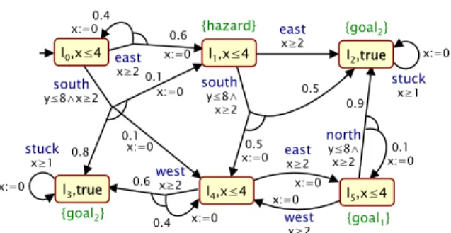
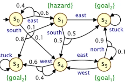
DRAFT The state spaces S of a DTMCD=(S,s,¯P,L) represent the set of all possible configurations of the system being modeled. Rr614.5[C6k] when1=(r1S,r1T),r1S(s)=1 ifis labeled risk and 0 otherwise andrT(s,s0)=0 for all,s0∈S– expected number of times the robot visits a labeled state of danger during the first steps is a maximum of 4.5. The main components of the model checking procedure are the calculation of the probability that a path formula is satisfied and the expected value of a reward formula.

The overall complexity of model checking is double exponential in formula and polynomial in DTMC size, but can be reduced to a single exponential. The second property can be expressed as the queryRr=?[Fdone], where the labels indicate the DTMC states where the calculation is complete, and the labels of the reward structure.

DRAFT

Stochastic Multi-Player Games

As for MDP, we can define a set of finite and infinite paths FPathsG (FPathsG(s)) and IPathsG (IPathsG(s)) from G. To resolve non-determinism in SMG, we reuse strategies, but now define a separate strategy for each player in the game. If a combined strategyσ is constructed from all playersΠ of group G (sometimes called a strategy profile), then the indeterminism is resolved in all states of the game and, as for MDP, we can construct probability measures PrσG, over the infinite paths of group G.

To specify properties of SMGs, we consider an extension of the PRISM logic previously used for DTMCs and MDPs, adding the coalition operatorhhCiifrom al-. Intuitively, the formulas neehhCiiP./p[ψ]andhhCiiRr./q[ρ] mean that it is possible for the players inC to jointly ensure that P./p[ψ]orRr./q[ρ] are satisfied, respectively, no matter what what the other players in the game decide to do. We can also adapt these to numerical queries, writing, for example, hhCiiPmax=?[ψ] to represent the maximum probability of ψ that the players iCcan ensure, regardless of the choices of the other players in the game.

Tool Support

• Controller Synthesis
• Controller Synthesis for MDPs

For this, we use a slightly different form of the satisfaction relation|=, where we write M,σ,s|=φto state that the property φ is satisfied by MDPM under strategyσ (which is essentially the same as satisfying eφunder DTMCMσ of induced). The problem of strategy synthesis is: given an MDP M with initial state ¯ and a formulaφ of the form P./p[ψ]or Rr./q[ρ] (see definition 3.3), find, if it exists, a strategyσ∗ ∈ΣM such thatM ,σ∗,s¯|=φ. 3.2.2, the strategy synthesis problem for the operator aP./p[ψ] orRr./q[ρ] can be solved by computing the suboptimal value (ie, the minimum or maximum value) for ψ orρ.

So, in general, rather than fixing a specific boundp, we can just use a numerical query like Pmin=?[ψ] to specify a strategy synthesis problem, and directly calculate an optimal value and strategy for it . For probabilistic reachability questions Pmin=?[Fa] orPmax=?[Fa], memoryless deterministic strategies reach optimal values, and thus this class of strategy is sufficient for strategy synthesis. Determining optimal probability values ​​requires an analysis of the underlying graph structure of the MDP, followed by a numerical calculation phase using, for example, linear programming, policy iteration or value iteration.

The construction of an optimal strategy σ∗ then depends on the method used in the numerical calculation phase. Policy iteration is the most direct because an optimal strategy is constructed as part of the algorithm. Strategy synthesis and the calculation of optimal reachability probabilities for step-by-step reachability is equivalent to working backwards through the MDP and determining at each step the actions that yield optimal probabilities in each state.

Example 5. Returning to our working example, we consider strategy synthesis for the queryRmovesmin=?[Fgoal2]where the movereward structure returns 1 for all state-action pairs and all state rewards are zero. We now consider strategy synthesis for a numerical query of the form Pmin=?[ψ] or Pmax=?[ψ], where ψ is the LTL formula. For a given MDPM, the problem can be reduced to the synthesis of a reachability query strategy (see Section 3.3.1.1) on the product M and a deterministic Rabin automaton (DRA) representing ψ[36].

Example 6. Returning again to the working example of the robot (Figure 3.4), consider the synthesis of a strategy for the query Pmax=?[ (G¬hazard)∧(G Fgoal1).

Multi-objective Controller Synthesis

For example, instead of synthesizing a strategy that satisfies P./1p1[ψ1]∧P./2p2[ψ2], we can instead find a strategy that maximizes the probability of satisfying the path formula ψ1 while simultaneously satisfying P./2p2[ψ2 ]. The method outlined above using linear programming can easily be extended to handle such numerical queries by adding an objective function. Pareto Queries. To analyze the trade-off between multiple objectives, we can construct the corresponding Pareto curve an approximation of it [46].

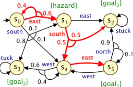
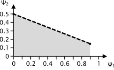
Recall that in Example 6 we considered the numerical query Pmax=?[ (G¬hazard)∧(G Fgoal1) ] and found that the optimal probability was 0.1. Instead, we consider each conjunction of the LTL formula as a separate objective and, for ease of notation, let ψ1=G¬hazard and ψ2=G Fgoal1. Consider the numerical multi-objective query that maximizes the probability of satisfying ψ2 while satisfying P>0.7[ψ1].

Finally, the Pareto curve for maximizing the likelihood of LTL formulas ψ1 and ψ2 is presented in the figure. The dashed line in the figure forms the Pareto curve, while the gray shaded area below shows all points (x, y) for which there is a strategy satisfying P>x[ψ1]∧P>y[ψ2].

Modelling and Verification of Large Probabilistic Systems

• Compositional Modelling of Probabilistic Systems
• Compositional Probabilistic Model Checking
• Quantitative Abstraction Refinement
• Case Study: The Zeroconf Protocol
• Real-Time Probabilistic Model Checking

We begin by defining the underlying concepts and then illustrate two of the rules of assumption-warranty-proof. The approach is based on the use of linear-time, action-based propertiesΨ, which are defined in terms of the actions that label the transitions of a probabilistic automaton (or MDP). This is in contrast to the properties discussed elsewhere in this chapter, which are defined in terms of the atomic propositions that label states.3.

See [81] for more details on the rules for accepting proof of warranty, including extensions to allow both ω-regular traits and reward-based traits. DRAFT aims to build a small abstract model, by removing details of the complex concrete system that are irrelevant to the property in question, which is consequently easier to analyze. The framework is used to verify or disprove properties of the form "the maximum probability of error is at most p" for a given probability threshold.

These bounds provide both a quantitative measure of the quality (or accuracy) of the abstraction and an indication of how to improve it. These probes are sent to all other hosts on the network and are used to check if any other devices are using the selected address. If the host does not receive a response to any of the probes, it starts using the selected IP address.

The model of this system studied in [81] consists of the parallel composition of two PAs: an automaton representing a new device joining the local network and the other representing the environment, i.e., in the case of the two final properties, the additions of rules in LTL and reward properties were used. The model is the parallel composition of 2·N+1 component PAs: the device that joins the network and N pairs of channels for two-way communication between the new device and each of the configured devices.

The graphs show how the differences between the lower and upper bounds can be used to quantify the usefulness of the abstraction.

Probabilistic Timed Automata

• Continuous-time Markov Chains
• Parametric Probabilistic Model Checking
• Parametric Model Checking for DTMCs
• Parametric Model Checking for Other Probabilistic Models
• Future Challenges and Directions

There are a number of different model checking approaches to PTA that support different classes of properties. It follows that the only difference between model control DTMCs and CTMCs concerns the finite property analysis. Model checking algorithms have been developed for such models, see for example [25], as well as.

In this section we consider another extension of the basic technique of probabilistic model checking that provides parametric techniques for analyzing models. We first consider the parametric model checking of DTMC models and, after this, consider approaches for other probabilistic models. Since then, further improvements to parametric model checking of DTMCs have been proposed [65], including the use of strongly coupled component decompositions and optimized approaches to the generation of rational functions; it was implemented in the PROPHECY tool [37].

Parametric probabilistic DTMC model verification has been applied to a variety of problems, including model repair [16] and sensitivity analysis [43]. Applying parametric probabilistic model checking results in the rational function (25·p·q+40·p−10·q−24)/(40·p−34) plotted for valid ranges of pandq in the figure. Parametric model checking techniques have also been developed for several of the other probabilistic models described in this chapter.

Parametric validation of unconstrained trait models for CTMC can use the same methods as those developed for DTMC. We should also mention [24, 26], which enables accurate parametric model verification of time-limited CTMC properties. The approach of [11] is based on an inverse method for parametric (non-probabilistic) time automata [10], while [69] extends forward accessibility [84] and game-based approaches [79] for PTA for model checking.

This chapter has provided an overview of probabilistic model checking and mapped some of the significant advances that have been made in the field in recent years. Probabilistic model checking has many applications in embedded and cyberphysical systems, for example in the verification of sensor networks or robotic applications. Counterexamples. A final challenge is to improve the quality and usability of the results generated by probabilistic model checking.