FACTORS DRIVING WEALTH INEQUALITY IN EUROPEAN COUNTRIES
Sebastian Leitner
177
MATERIALIEN ZU WIRTSCHAFT UND GESELLSCHAFT
978-3-7063-0736-9
WORKING PAPER-REIHE DER AK WIEN
WPR_177_Wealth Inequality.indd 1 26.06.18 13:25
Materialien zu Wirtschaft und Gesellschaft Nr. 177 Working Paper-Reihe der AK Wien
Herausgegeben von der Abteilung Wirtschaftswissenschaft und Statistik der Kammer für Arbeiter und Angestellte
für Wien
Factors driving wealth inequality in European countries
Sebastian Leitner
Juli 2018
Die in den Materialien zu Wirtschaft und Gesellschaft veröffentlichten Artikel geben nicht unbedingt die
Meinung der AK wieder.
Die Deutsche Bibliothek – CIP-Einheitsaufnahme
Ein Titeldatensatz für diese Publikation ist bei der Deutschen Bibliothek erhältlich.
ISBN 978-3-7063-0736-9
Kammer für Arbeiter und Angestellte für Wien A-1041 Wien, Prinz-Eugen-Straße 20-22, Tel: (01) 501 65, DW 12283
Factors driving wealth inequality in European countries
The effect of inheritance and gifts on household net wealth distribution analysed by applying the Shapley value approach to decomposition
by Sebastian Leitner†°
December 2017
Zusammenfassung
In der vorliegenden Studie werden mikroökonomische Ursachen für die Ungleichheit von Haushaltsvermögen in neun Ländern der Europäischen Union untersucht. Die Analyse basiert auf Mikrodaten des Eurosystem Household Finance and Consumption Survey (HFCS 2014) und wird mittels der sogenannten Shapley-Wert-Dekompositionsmethode durchgeführt. Die Forschungsergebnisse zeigen, dass Erbschaften und Schenkungen einen beachtlichen Effekt auf die gemessene Vermögensungleichheit haben; dieser ist im Schnitt stärker als der Einfluss vorhandener Einkommensdifferenzen. Ererbte Sach- und Finanzwerte tragen in Österreich, Deutschland, Frankreich, Portugal und Spanien 30% oder mehr zur gesamten, gemessenen Vermögensungleichheit bei. Gleichwohl prägt auch die Verteilung anderer sozioökonomischer Charakteristika der Haushalte innerhalb der Länder (Alter, Bildungsstand, Haushaltsgröße, Anzahl Erwachsener sowie Kinder im Haushalt und Familienstand) die beobachtete Vermögensverteilung. Die Untersuchungsergebnisse gleichen jenen einer Vorgängerstudie (Leitner, 2016) basierend auf Daten der ersten Welle des Household Finance and Consumption Survey (HFCS 2010).
Abstract:
This paper analyses how microeconomic factors drive the inequality in household wealth across nine European countries applying the Shapley value approach to decomposition. The research draws on micro data from the Eurosystem Household Finance and Consumption Survey 2014. Disparity in inheritance and gifts obtained by households are found to have a considerable effect on wealth inequality that is on average stronger than the one of income differences and other factors. In Austria, Germany, France, Portugal and Spain the contribution of real and financial assets received as bequests or inter-vivos transfers attains more or almost 30% to explained wealth inequality. However, also the distribution of household characteristics (age, education, size, number of adults and children in the household, marital status) within countries shapes the observed wealth dispersion. The results
resemble those obtained in a similar study (Leitner, 2016) based on data from the first wave of the Eurosystem Household Finance and Consumption Survey (HFCS 2010).
JEL classification: D31, D63, O52, O57
Keywords: Inequality, Wealth Distribution, Decomposition Analysis, Inheritance, Inter vivos transfers, Income Distribution, Europe
Research was financed by the Austrian Chamber of Labour.
† The Vienna Institute for International Economic Studies (wiiw); Rahlgasse 3, 1060 Vienna, Austria;
Email: [email protected]
° The author wishes to thank Stefan Jestl and many others for helpful comments and assistance.
1
Introduction
In recent years the topic of household wealth holdings and their distribution has been discussed intensively in the literature. An obvious reason for this is the increase of accumulated private wealth in relation to the national income in the affluent industrialised economies, from the late 1970s onwards as analysed among many others by e.g. Piketty (2014). In addition to this development, in most OECD countries inequality of income rose from the 1980s onwards (see for example OECD 2011).
Another reason for the increased interest in research on household wealth is that micro data have become available in the past two decades for more and more countries that allow us to study wealth holdings and inequality, not only at the level of individual countries but also to compare the situation across countries, first via the Luxembourg Wealth Study Database and more recently based on data from the Eurosystem Household Finance and Consumption Survey (HFCS).
In a previous paper (Leitner, 2016) I have already applied the Shapley value approach to decomposition to wealth inequality based on HFCS 2010 data. The present paper replicates the analysis using data from the second wave of the survey (HFCS 2014). Thus the aim is to test the robustness of the results obtained previously and analyse potential differences. Similar to the previous research done (Leitner, 2016), my assumption is that the accumulation of wealth stocks by households is facilitated by the receipt of bequests or gifts (mostly of ancestors). Thus the wealth inequality of one generation can be passed on to the following, which over longer periods of time may result in an increase in the inequality of wealth within a society. In principle, households build up wealth stocks in three ways. Either they save out of their income from employment or self-employment or out of financial sources. The second way, important for many households, is to receive bequests or gifts and to save them instead of using the assets for consumptive purposes. A third form, which however cannot be dealt with in this paper, is that the assets owned appreciate in real terms. In my paper I am interested in the process of households’ building-up of wealth stocks via the first two processes and the respective inequality in asset holdings that results therefrom. In order to detect the sources of wealth inequality across countries I apply (as in Leitner, 2016) a decomposition methodology based on the Shapley value approach to the inequality measure used most frequently in the literature: the Gini index. This decomposition method allows for an assessment of the relative importance of explanatory factors in inequality. While some authors (see the literature review below) have already worked for some decades on measuring how much of the accumulated stock of household wealth can be attributed to inheritance and intergenerational inter vivos transfers (contrary to wealth built up over the life cycle via saving and investment), decomposition approaches to the distribution of wealth have been performed only recently. However, in the literature one can so far find only decompositions by wealth source but not by subgroups. This latter analysis is performed in the following and should highlight the relative importance of inheritance, income and household characteristics in shaping wealth inequality in a cross-country manner, thus providing a novel contribution to the literature.
The paper is organised as follows: Since the approach of this paper equals the one of previous research performed in Leitner (2016) I will not replicate or present a distinct literature review in this publication.
Instead I refer the reader to the one presented there, covering the relevant publications on developments of household wealth inequality, the effects of inheritance and inter vivos transfers and on decomposition methods used to analyse income and wealth inequality. Section 2 discusses the most relevant aspects of the data used (sources, measurement issues and definitions) and Section 3
2
introduces the concept of the Shapley value approach to decomposition, discussing the way I apply this method. Section 4 presents the empirical results of the analysis for inequality in net wealth stocks of households and Section 5 compares those with previous outcomes based on HFCS 2010 data as published in Leitner (2016). Section 6 concludes.
Data
The data for the analysis presented in this paper are drawn from the Household Finance and Consumption Survey wave 2 (HFCS 2014 – UDB 2.0). Furthermore the results were compared to those published in Leitner (2016) were analysis was performed using data from the first wave of the survey (HFCS 2010 - UDB 1.1 published in February 2015). While in the first wave the survey was conducted in 15 euro area countries1, in the second wave not only all euro area countries except for Lithuania participated, but also Hungary and Poland. Due to data issues however not all of these countries could be considered in the analysis presented in this paper. A detailed description of the methodology of the survey is presented by the European Central Bank (2016). The HFCS provides data on gross and net wealth holdings of households and their components and socioeconomic characteristics for the households and their individual members. Moreover, it covers data on inheritance and gifts received and gross income. Interpreting results in cross-country comparisons of wealth inequality should be done cautiously. As discussed by, for example, Fessler/Schürz (2013) and Tiefensee/Grabka (2014) and more recently Fessler/Lindner/Schürz (2016), although a lot of ex-ante harmonisation was conducted, there are several aspects of potential methodological constraints regarding cross‐country comparability due to non-harmonisation of sampling frames, sample sizes, survey modes, oversampling of top wealth households, reference periods, weighting or imputation methods applied and variations in initial response rates by countries. Nevertheless, as emphasised by Tiefensee/Grabka (2014:26), ‘the HFCS is still the best dataset for cross-country comparisons of wealth levels and inequality in the Euro area and it is definitely a first (big) step into the right direction’. The HFCS data offer five different multiple imputations in order to correct for item non-response. I take these imputations into account in my estimation analysis by using Rubin’s Rule. Moreover, unit non-response is accounted for in the HFCS data by providing 1000replicate weights, which are all used in my estimations.
Similar to the analysis performed in Leitner (2016) in this paper I also decompose two different variables depicting wealth holdings of households: gross wealth (total household assets excluding public and occupational pension wealth) and net wealth (gross wealth minus total outstanding household liabilities).
As explanatory variables I first apply total household gross income and five different types of inheritances and gifts (household main residence, further dwellings, land, business and the sum of other assets) received by all household members. Obviously, the net income of households would be a better measure of assessing the potential of households to save out of their income; moreover, present income may not be the best predictor of income flows accrued by individuals in their previous (working) life; however, this information is so far not available in the HFCS. In the HFCS 2014, the reference person is asked to provide information on whether the main household residence, if owned, was inherited or a gift. Furthermore, information is collected on up to three inheritances or substantial gifts from someone who is not a part of
1 The HFCS 2010 was conducted in Austria, Belgium, Cyprus, Finland, France, Germany, Greece, Italy, Luxembourg, Malta, the Netherlands, Portugal, Spain, the Slovak Republic and Slovenia.
3
the current household. Since in the case of Finland no data were provided on inheritances and for the Netherlands, Cyprus and Greece the share of households having provided information on inheritances (and gifts) received were considerably low, I had to exclude those three countries from the analysis. Malta could not be included in the analysis either, owing to multiple data problems. In general, inheritance data have to be interpreted cautiously as inheritances are notoriously underreported in wealth surveys. The rate of refusal to answer questions concerning inheritances especially rises in line with the wealth holdings of households (Fessler/Schürz 2013). Most probably this results in an underestimation of wealth inequality.
It should be pointed out that bequests and gifts acquired in the past are not automatically part of the actual present wealth stock. In the period between acquisition and the time of the survey interview, assets may have been used not only for the accumulation of the wealth stock of the household, but, for example, also for consumption purposes or inter-household transfers. Thus a regression of wealth stocks on wealth transfers received is not a means of explaining the total sum of wealth by its parts.
In addition to the value of the property at the time of acquisition (by way of inheritance or gift), information is collected on the date of acquisition. In order to make the assets inherited or acquired as gifts comparable with each other both within households and between households, we have to calculate the present value of the assets. The problem is dealt with in different ways in the literature; the resulting assumptions differ between a depreciation of the real value of assets (by leaving the nominal value of the acquired asset unchanged) and an appreciation of up to 3 per cent annually. For the lack of information on actual appreciation I resort to the conservative method applied by, for example, Fessler et al. (2008a; 2008b) and Fessler/Schürz (2013), assuming the retention of the real value of the asset by appreciation, using the annual national consumer price index (CPI). The data were provided by the AMECO database from 1960 onwards for all euro area countries except for those being EU New member states (NMS), i.e. Estonia, Latvia, Slovak Republic and Slovenia. Data from 1960 onwards was available for Poland, but not for Hungary. Thus all NMS except Poland had to be excluded from the analysis as well. For assets acquired before 1960 I have to assume no increase in value up to1960. Of those households having received inheritances and gifts, 1.8 per cent acquired them before 1960 (unweighted average over shares of countries analysed). Concerning the application of the CPI for the calculation of the present value of the assets inherited or received as gifts I do not differentiate between different kinds of assets since households could swap between asset types. However, in the regression analysis I use the information of asset types to construct different explanatory variables. In the case of dwellings, land and businesses (including securities and shares) acquired, I assume that households have a higher incentive to keep those assets and further invest in them, and that those assets appreciate with an interest rate exceeding the CPI (the applied appreciation rate for bequests and gifts) resulting in higher wealth stocks of households having inherited those assets. Thus the present value of the following groups of assets acquired via inheritance (or as gift) were used as separate explanatory variables: household main residence; dwellings apart from household main residence and use of dwellings; land; businesses (including farms), securities and shares; further assets inherited (or received as gifts). The latter group of assets also includes the values of those inheritances (or gifts) which comprise more than one specific asset, since in such cases the value of individual assets is not provided for in the HFCS data file.2 Some information that was used as an additional explanatory variable
2 In the case of France, only 63 per cent of the present value of inheritances and gifts could be assigned to one of the five specific groups of assets described above (that is, the rest of the value had to be assigned to the category ‘other assets’). For further countries analysed: LU: 71 per cent, PT: 79 per cent, AT: 84 per cent, DE: 84 per cent, ES: 85 per cent, IT and PL: 100 per cent.
4
was not collected in all euro area countries. This was the case for the question of expectations on the receipt of a substantial gift or inheritance in the future for Spain.
Furthermore, I use socioeconomic characteristics as explanatory variables. For this I employed personal characteristics of the household members in order to construct variables for the household level. These are: the household level of educational attainment; the aver-age age of adult household members (being more than 19 years of age); and the household size, that is to say the number of adults and children in the household. Moreover, I used dummies for the marital status of the household reference person (being single, married, widowed, divorced or living in a consensual union on a legal basis). The reference person of the household provided in the HFCS – UDB 1.1 data file version (variableDHIDH1) is chosen according to the ‘Canberra’ definition.3 The household level of educational attainment is calculated as the average attainment level (expressed in average years of schooling needed to attain the education level stated for the individual household members)of all household members above the age of 16 and no longer in education (and thus potentially available for the labour market). The use of socioeconomic characteristics is particularly important in the case of cross-country comparisons since differences in household structures have a substantial effect on the measured summary statistics of wealth distribution in the euro area (see for example Fessler et al. 2014). For instance, I expect that households with more members, with higher average education levels and whose members have a higher average age tend to possess higher stocks of household wealth.
Methodology
The methodology of the Shapley value approach to decomposition applied in this paper has already been explained in detail in Leitner (2016). However, in order to make the analysis more user-friendly, we will repeat the explanation in the below. The advantage of a regression-based approach is that the relative importance of many variables and groups of them to explain inequality (socioeconomic characteristics of individuals or households such as age, gender, educational attainment, employment status, but also decisive monetary values such as income, etc.) is taken into account simultaneously.
Thus, the regression approach (step 1) allows assessing the importance of each of these explanatory variables conditional on all other variables for any dimension of inequality considered (in our case stocks of household net and gross wealth). The Shapley value approach (step 2) then further allows calculating the contribution of each of these explanatory variables to the respective inequality measure.
The Shapley value approach can be illustrated by using a simple example with three explanatory variables. We first regress individual wealth levels y on these explanatory variables xi (i1,2,3),
0 1x1 2x2 3x3
y ,
where
denotes the error term. The predicted wealth level is then given by
3 The procedure of identification of the reference person is described in United Nations Economic Commission for Europe (2011: 65).
5
ˆ . ˆ ˆ
ˆ123 ˆ0 1x1 2x2 3x3 y
This predicted value is then used to calculate the Gini coefficient
G ˆ
1230 , where subscripts denote the variables included. In the first round we then eliminate one variable and calculate the predicted wealth levels yˆ 23,yˆ 13 and yˆ 12 for each household using the vectors of xi and the original coefficients
ifrom our wealth estimation (see step 1 of the approach). The corresponding Gini coefficients are then given by Gˆ 123,Gˆ 131 and Gˆ 121 respectively. Analogously, in a second round we eliminate two variables, thus calculating yˆ 1 ,yˆ 2 and yˆ 3 . The resulting Gini coefficients are
G ˆ
12, G ˆ
22 and Gˆ 32 . The final round would then be to include the constant only; the resulting Gini coefficient would thus be
0 . ˆ
3 G
The marginal contributions are then calculated using the Gini coefficients. The first round marginal contributions for each variable are
C
1(1) G ˆ
(1230) G ˆ
(231) ,C
2(1) G ˆ
(1230) G ˆ
(131) and (121) )
0 ( 123 )
1 (
3
G ˆ G ˆ
C
.The marginal contributions in the second round of the first variable are given by
(22) )
1 ( 12 ) 1 , 2 (
1
G ˆ G ˆ
C
andC
1(2,2) G ˆ
(131) G ˆ
(32)The average of these contributions is the marginal contribution of the first variable in the second round, i.e.
1 2,2
1 , 2 1 )
2 (
1 2
1 C C
C . Similarly we calculate C2 2 and C3 2. The third round contribution is given by
C
1(3) G ˆ
(12) G ˆ
(3) G ˆ
(12) asG ˆ
(3) 0
and analogously for C2(3) Gˆ (22) and (32) ) 3 (
3 Gˆ
C .
Finally, averaging the marginal contributions of each variable over all rounds j 1,2,3 results in the total marginal effect of each variable, i.e.
1 2 3
3 1
j j
j
j C C C
C .
The proportion of inequality not explained is then given by
(1230)
Gˆ G
CR .
The approach can easily be extended to any number of explanatory factors and to other inequality measures. However, since the number of combinations and thus Gini coefficients to be calculated grows exponentially with the number of variables, in practice is it necessary to combine the variables to seven or eight explanatory factors in order to keep the necessary computing time tolerable. In our case we included in the explanatory factor inheritance the effect of the individual types of bequests and gifts and the effect of expected inheritance; the factor household age includes the variable household age and household age2, household structure includes the effect of both the variables number of adults and number of children and the explanatory factor marital status comprises the
6
effect of all three dummy variables for single, widowed and divorced reference persons of households (comparing their wealth holdings with those of reference persons being married or living in a consensual union).
Wan (2002) points to the fact that the presence of a negative constant in the regression equation may lead to negative predicted individual income levels. In that case the calculation of a Gini coefficient and thus the contributions of individual variables to overall inequality would be impossible. To overcome this pitfall he shows in Wan (2004) that different model specifications can be used for the underlying estimated income (in our case wealth) generating function, delivering moreover better log- likelihood values than the linear estimation model. Following his approach, we choose for the analysis in this paper a semilog model:
0 1 1 2 2 3 3
ln y x x x . (1)
Since the distribution of wealth data is not only highly skewed but net wealth data also comprise, due to outstanding debts of households, negative and zero values we cannot apply a logarithmic transformation of the data but resort to a transformation often used in the literature on wealth stocks (see e.g. Burbidge et al., 1988; MacKinnon and Magee, 1990; Pence, 2006; Schneebaum et al., 2014) – the inverse hyperbolic sine transformation (IHS):
( i) ln i i2 1
i IHS W W W
y . (2)
This transformation is used not only for the wealth stocks but also the calculated sums of inheritances and gifts and the income of households since both can also feature zero and the latter for self- employed income also negative values. Thus our semilog model takes the form:
ln 2 1 0 1 1 2 2 3 3
ln y W W x x x . (3)
Since we are not interested in the decomposition of the log of wealth, but wealth in nominal terms, in the second step of the decomposition analysis we calculate the fitted values for the wealth levels of households after taking the antilog of the above model, resulting in:
i i
ii
x x
y x
e e
e e
elnˆ ˆ0 ˆ1 1 ˆ2 2 ˆ3 3 , (4) where ˆi denotes the coefficients of the estimated regression (3). In our case, after the above- described IHS transformation, this results in
xi xi
xii i
i W W e e e e
yˆ ˆ ˆ2 1 ˆ0 ˆ1 1 ˆ2 2 ˆ3 3 . (5) The advantage of this model is that in this case the constant eˆ0 becomes now a positive scalar which does not influence the magnitude of the calculated Gini coefficient. The elimination procedure as described above however remains unchanged. As one can see, we approximate wealth inequality with the transformed fitted values of the household wealth levels Wˆi Wˆi2 1 stemming from
) ˆ 1 ln(Wˆi Wi2
e instead of Wˆi. This would only be problematic if we had a large number of negative
7
predicted values. However, since in our sample this is only the case in about 4% of the cases (with mostly low absolute values) the inequality levels calculated are almost the same based either on
ˆ 1 ˆi Wi2
W or Wˆi.
Empirical results
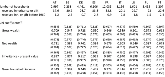
In order to describe the situation of wealth distribution in the analysed countries, we start by taking a look at the inequality of wealth and income across countries. Table 1 presents the Gini indices of wealth of households. We can observe that both gross and net wealth are distributed much more unequally compared to household gross income. Moreover, the Gini indices for household wealth are much higher in Germany and Austria, while lowest in the group of countries analysed in this paper in Poland, Belgium and Spain. Bequests and gifts at present value are even more unequally distributed than net wealth. Taking into account the underreporting of inheritances, the inequality of bequests may be even higher. This is an effect of the relatively low rates of households having acquired an inheritance (or substantial gift) up to the date of the survey. In Italy only an estimated 20.1% of all households received bequests, while in Austria and France the share is 37.6% and 38.8%, respectively.
Table 1: Descriptive statistics of inheritance and gifts, gross and net wealth and household income
AT BE DE ES FR IT LU PL PT
Number of households 2,997 2,238 4,461 6,106 12,035 8,156 1,601 3,455 6,207 received inheritance or gift 37.6 30.2 26.7 33.6 38.8 20.1 29.7 23 22.6
received inh. or gift before 1960 1.2 2.5 0.7 2.8 0.9 2.8 1.8 1.5 2.4
Gini coefficients1)
(0.654) (0.528) (0.711) (0.528) (0.627) (0.574) (0.569) (0.562) (0.597)
Gross wealth 0.709 0.547 0.728 0.550 0.646 0.589 0.601 0.573 0.613
(0.764) (0.566) (0.746) (0.573) (0.665) (0.605) (0.633) (0.585) (0.630) (0.678) (0.570) (0.746) (0.575) (0.659) (0.587) (0.615) (0.574) (0.663)
Net wealth 0.731 0.589 0.762 0.599 0.676 0.603 0.646 0.587 0.678
(0.784) (0.607) (0.777) (0.623) (0.694) (0.619) (0.677) (0.600) (0.693) (0.869) (0.861) (0.897) (0.898) (0.885) (0.930) (0.877) (0.993) (0.942) Inheritance - present value 0.897 0.874 0.917 0.929 0.907 0.940 0.898 0.997 0.956 (0.925) (0.886) (0.937) (0.96) (0.928) (0.950) (0.919) (1.000) (0.970) (0.336) (0.368) (0.429) (0.419) (0.365) (0.402) (0.404) (0.389) (0.418) Gross household income 0.349 0.392 0.449 0.437 0.374 0.416 0.417 0.401 0.437 (0.362) (0.416) (0.468) (0.454) (0.383) (0.430) (0.430) (0.414) (0.456)
Note: 1) Lower and upper bounds of 95% confidence interval in parentheses.
Source: HFCS 2014 - UDB 2.0, wiiw calculations.
Regression analysis
The Shapley value decomposition approach described above requires first to regress the IHS-transformed net wealth level of the households on the explanatory variables. In our case these are first the IHS- transformed (calculated) present values of five different groups of specific asset types inherited or acquired
8
as gifts. Further explanatory variables are a dummy for the expectation of future substantial bequests or gifts, gross household income and a set of socioeconomic characteristics4: the average age of the household members (and the square of this variable), the average education level of household members and the number of adults and children in the household. Moreover, we apply dummies for the marital states of the reference person of the household. We expect wealth of households to increase conditionally on amounts of inheritances (and substantial gifts) acquired and household gross income respectively.
The results presented in Table 2 below show that in general the coefficients have the expected signs and are significant for a large part of the explanatory variables in most countries. The explained part of the variance amounts to 20% on average (unweighted over countries) as shown by the R². For those three asset types being most important in the total value of inherited wealth on average (household main residence, land and further dwellings) the positive conditional correlation with net wealth is highest for Germany and Austria. All inherited asset types are positively correlated with net wealth if coefficients are significant. Almost all results are significant, with the only exceptions of inherited money in the case of Spain, land in the case of Belgium and Luxembourg, businesses securities and shares also in the of Belgium, Luxembourg and Italy; furthermore in the case of Poland the coefficient for asset types not specifically classified (‘Other assets’) is not significant. The expectation of a substantial gift or inheritance is a robust conditional predictor of higher net wealth values only in five out of the nine countries analysed. For income the regression results are obviously very robust.
Households with higher earnings tend to be wealthier.
The higher the average age of the household, the more the members had time to accumulate wealth.
Coefficients for age and age² show that household net wealth rises with increasing average age of the (adult) household members; however no significant results concerning age could be found for Austria.
For most countries on average the peak of wealth is reached between 55 and 65 years (average age of adult household members). Households with higher average education levels hold conditionally higher net wealth, a robust result in all countries but Luxembourg. In general, larger households seem to have the possibility to accumulate higher wealth. More children in the household in general correlate with lower levels of net wealth. However, only in the case of Austria and Portugal the coefficients are significant. As expected, households where the reference person is married or lives in a consensual union have conditionally higher wealth compared to all other households. For completeness we should also mention here that in an earlier version of the regression model we included also the gender of the reference person as an explanatory variable and the share of female members in households.
However, the results were non-significant.
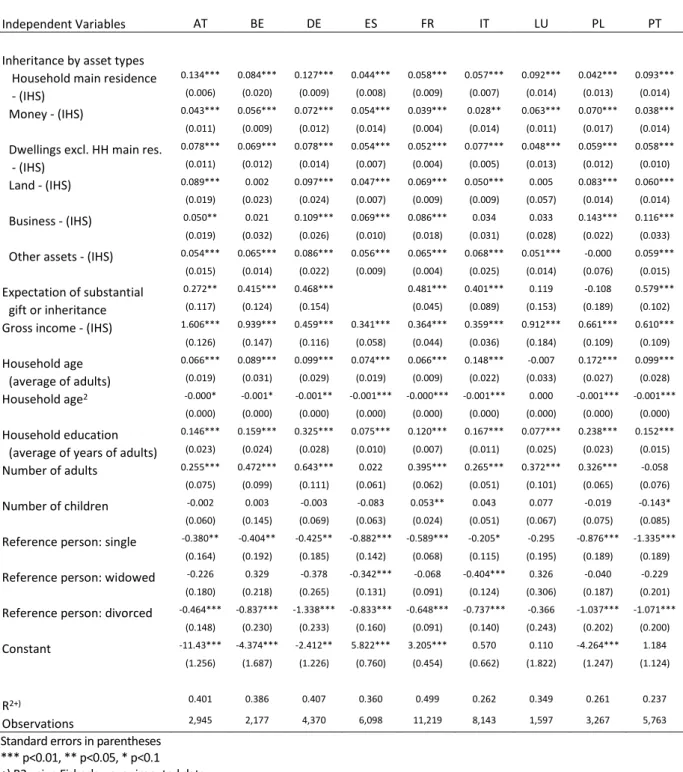
In addition to net wealth of households we also regress gross wealth levels on the above-described explanatory variables. The results are presented in Table A.1 in the appendix and are not discussed in detail here. However, described in brief they are similar to those with respect to household net wealth. Coefficient signs remain in general the same, whilst the share of the explained variance increases to an R² of some 35%.
This is no surprise since the underlying decisions of households to borrow money for private or business purposes are influenced by reasons more difficult to be described with the information available from the
4 Obviously one could apply different explanatory variables particularly for detecting the influence of
household characteristics. In a robust check we also used alternatively the household type dummies applied by Fessler et.al. (2014). The results concerning the contributions of inheritance and gifts, income and education remained robust. The advantage of our set of explanatory variables is that we can identify the individual effects of age, number of adults and children and marital status of reference persons, which are in the case of the above mentioned household type dummies intermingled.
9
HFCS, thus the individual amounts of net wealth are more difficult to be estimated compared to gross wealth. Regression results in general show (see Table A.1), that the signs of the coefficients do not change, compared to the regression results based on net wealth, and are significant in more cases. The size of the coefficients decline for most variables unsurprisingly, since the values of individual household gross wealth are obviously higher than the ones of net wealth.
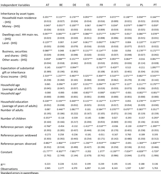
Table 2: OLS estimations predicting IHS transformed household net wealth
Independent Variables AT BE DE ES FR IT LU PL PT
Inheritance by asset types
Household main residence 0.201*** 0.115*** 0.176*** 0.093*** 0.070*** 0.072*** 0.138*** 0.058*** 0.166***
- (IHS) (0.013) (0.027) (0.024) (0.014) (0.016) (0.009) (0.021) (0.015) (0.019) Money - (IHS) 0.045* 0.055** 0.100*** 0.067 0.046*** 0.034* 0.079** 0.088*** 0.059*
(0.026) (0.023) (0.033) (0.052) (0.009) (0.019) (0.031) (0.025) (0.033)
Dwellings excl. HH main res. 0.097*** 0.085*** 0.138*** 0.086*** 0.071*** 0.092*** 0.051* 0.086*** 0.078**
- (IHS) (0.023) (0.019) (0.020) (0.011) (0.008) (0.006) (0.026) (0.015) (0.031) Land - (IHS) 0.129*** 0.007 0.144* 0.061*** 0.093*** 0.062*** 0.004 0.120*** 0.103***
(0.035) (0.030) (0.079) (0.016) (0.010) (0.010) (0.077) (0.017) (0.022)
Business, securities 0.088*** 0.048 0.186*** 0.131*** 0.114*** 0.039 0.056 0.178*** 0.172***
and shares - (IHS) (0.029) (0.044) (0.048) (0.020) (0.022) (0.037) (0.048) (0.027) (0.042) Other assets - (IHS) 0.059* 0.088*** 0.151*** 0.073*** 0.082*** 0.093*** 0.064** -0.016 0.081***
(0.034) (0.018) (0.042) (0.019) (0.010) (0.035) (0.026) (0.114) (0.028)
Expectation of substantial 0.145 0.630*** 0.994** 0.729*** 0.429** 0.515 -0.211 1.095***
gift or inheritance (0.389) (0.190) (0.392) (0.108) (0.167) (0.401) (0.334) (0.233) Gross income - (IHS) 2.319*** 1.237*** 0.483*** 0.325*** 0.304*** 0.510*** 1.071*** 0.682*** 0.543***
(0.258) (0.260) (0.165) (0.084) (0.049) (0.062) (0.270) (0.136) (0.142)
Household age 0.065 0.096** 0.105* 0.331*** 0.094*** 0.181*** 0.127* 0.211*** 0.170***
(average of adults) (0.045) (0.047) (0.057) (0.077) (0.019) (0.033) (0.073) (0.036) (0.052) Household age2 -0.000 -0.000 -0.000 -0.002*** -0.000* -0.001*** -0.001 -0.002*** -0.001**
(0.000) (0.000) (0.001) (0.001) (0.000) (0.000) (0.001) (0.000) (0.000)
Household education 0.228*** 0.193*** 0.449*** 0.115*** 0.132*** 0.179*** 0.055 0.278*** 0.193***
(average of years of adults) (0.052) (0.038) (0.052) (0.025) (0.013) (0.017) (0.054) (0.029) (0.030) Number of adults 0.087 0.446** 1.081*** 0.101 0.584*** 0.370*** 0.670*** 0.383*** 0.351**
(0.195) (0.186) (0.222) (0.167) (0.105) (0.071) (0.156) (0.119) (0.159)
Number of children -0.353** -0.118 -0.339 -0.145 -0.084 0.027 -0.293 -0.157 -0.293*
(0.164) (0.166) (0.217) (0.204) (0.053) (0.069) (0.192) (0.136) (0.163)
Reference person: single -0.766* -0.454 -0.132 -1.413*** -0.518*** -0.036 -0.130 -0.959*** -1.399***
(0.393) (0.285) (0.437) (0.444) (0.154) (0.170) (0.401) (0.258) (0.355)
Reference person: widowed -0.273 0.258 -0.236 -0.181 -0.011 -0.167 0.760 -0.189 0.193
(0.303) (0.392) (0.443) (0.254) (0.171) (0.142) (0.480) (0.250) (0.312)
Reference person: divorced -0.882** -1.866*** -2.019*** -1.236*** -0.919*** -0.866*** -0.691 -1.369*** -1.828***
(0.352) (0.534) (0.490) (0.427) (0.196) (0.250) (0.536) (0.312) (0.466)
Constant -21.77*** -9.302*** -7.801*** -3.202 1.377* -3.139*** -7.024** -6.828*** -3.729*
(2.792) (2.749) (2.144) (2.679) (0.741) (0.986) (3.044) (1.673) (1.906)
R2+) 0.223 0.228 0.215 0.199 0.239 0.195 0.145 0.188 0.136
Observations 2,945 2,177 4,370 6,097 11,143 8,143 1,597 3,267 5,763
Standard errors in parentheses
*** p<0.01, ** p<0.05, * p<0.1 +) R2 using Fisher's z over imputed data Source: HFCS 2014 - UDB 2.0, own calculations.
10
Shapley value decomposition
Now we turn from the explanation of wealth levels of household to the explanation of wealth inequality levels in individual countries by applying the Shapley value approach to inequality decomposition. Figure 1 presents the decomposition results for net household wealth. First we see that the Gini index calculated from the predicted values of the wealth generating function is somewhat higher to the one based on the original wealth data on households. In the case of France wealth inequality is overestimated by about 10%, for Poland by about 35%. Looking into the detailed results for net wealth by quantiles, we can detect that the highest relative differences between predicted and original values are between the 40th and 60th percentile for most countries. Here we tend to underestimate the levels of net wealth. Thus the cross- country comparisons of absolute contributions of explanatory variables to the Gini coefficient have to be interpreted with care, while the comparison of the shares in the explained (calculated) inequality (see Figure2) is less problematic.
Figure 1
From the explanation of the methodology above one can derive that the extent to which an explanatory factor or variable contributes to the Gini coefficient depends, first, on the dispersion of wealth between the household subgroups being defined by the characteristics described by the variables and, second, on the shares of the subgroups in the total population. In our case in order to keep the computing time of the Shapley value analysis tolerable we collapsed the effects of the individual types of bequests and gifts and the effect of expected inheritance to the explanatory factor inheritance and gifts; the factor household age includes the variables household age and household age2; household structure includes the effect of both the variables number of adults and number of children and the explanatory factor marital status comprises the effect of all three dummy variables for single, widowed and divorced reference persons of households.
-0,3 -0,2 -0,1 0,0 0,1 0,2 0,3 0,4 0,5 0,6 0,7 0,8 0,9 1,0
PL BE ES IT LU FR PT AT DE
Residual (unexplained) Ref. person: Marital status HH structure
HH av. education HH av. age HH income
Inheritance and gifts Gini-Index
Source: HFCS 2014 - UDB 2.0, wiiw calculations.
Shapley value decomposition - net wealth
contribution of groups of explanatory variables to Gini index
Gini index
11
In the case of the decomposition of net wealth we can observe that for the countries analysed on average almost 47% of the wealth inequality can be explained by the variation of gross income and acquired bequests and gifts (see Figure 2). Thus the differences in the accumulation of wealth are also significantly driven by the variations in household characteristics. However, the results differ strongly between countries. In the majority of countries and particularly those with the highest levels of inequality of net wealth the inequality of inheritances is the most important driver of overall wealth dispersion. In Germany and Austria (see Figure 1) more or almost 0.3 of the Gini index stems therefrom. However, in relative terms (as a share of the overall explained inequality) also in the case of Portugal, France, Spain and Poland, the latter country featuring the lowest level of dispersion in net wealth, more than 30% of the Gini coefficient can be explained by the inequality of inheritances. In the rest of the countries analysed, inheritances explain between 20% and 25% of the Gini index.
A noticeable divergence between Austria, Belgium and Luxembourg on the one hand and all other countries analysed can be observed in the case of the contribution of household gross income. In Austria household income explains even 35% of the inequality level, in both Belgium and Luxembourg 26%. The average contribution for all other EU members analysed amounts to only 11%.
Figure 2
Smaller differences can be detected according to the contributions of the average education level of households. In general the relative contributions fit well to the differences in dispersion of household education levels across countries. Within the European Union, Portugal features the highest level of inequality in educational attainment rates (see e.g. Leitner and Stehrer, 2014), while particularly low dispersion according to this characteristic is to be found in Austria. Also the ranking of the other countries in the Shapley decomposition corresponds with the one according to educational inequality between households, with the exception two countries. In Portugal, Poland and Italy the dispersion in education explains somewhat above 20% of the Gini index, in France, Belgium and Spain between 15% and 18%, in Austria only 10%. Luxembourg and Germany are exceptions concerning the contributions of household education. In the former it is with only 4% surprisingly low, while in latter with 20% rather high, although
0,0 0,1 0,2 0,3 0,4 0,5 0,6 0,7 0,8 0,9 1,0
0 10 20 30 40 50 60 70 80 90 100
PL BE ES IT LU FR PT AT DE
Ref. person: Marital status HH structure
HH av. education HH av. age HH income
Inheritance and gifts Gini-Index (right scale)
Source: HFCS 2014 - UDB 2.0, wiiw calculations.
Shapley value decompositon - net wealth
contribution of groups of explanatory variables to explained inequality, in %
Gini index
12
the dispersion of average household education levels is very low in Germany. That means that in Luxembourg households with relative low educational background possess relatively high levels of net wealth and vice versa, while in Germany the distribution of average household education levels overlaps very well with the distribution of net wealth values among households.
In the case of the average age of the household members, one can see that the contribution to total inequality does not only depend on the conditional effect age has according to the regression analysis on wealth levels. Also the differences between countries in the actual age structure of the population and thus the relative size of the age groups influence the decomposition results. In France and Spain the contribution of age is quite high, adding between 25% and 30% to the Gini index, while in Luxembourg and Italy it is still above 20%. In all other countries variation by average age of adult household members is contributing less strongly to overall wealth inequality, between 12% and 17%. As we could already expect from the underlying regression analysis, net wealth does not significantly differ conditional on all other explanatory variables between households of different size in Austria and Portugal. Hence, the size of the contribution amounts to 2.9% and 3.6% in those two countries. In Poland, France, Germany and Luxembourg differences in the structure of households are more important in explaining wealth inequality, the contribution ranges between 10% and 15% of the explained inequality. Wealth differences due to the marital status of the reference person are relatively low in Italy, Austria and Germany (ranging between 4% and 5%). In all other countries the contribution ranges between 7% and 10%.
A subsequent step in the analysis is the decomposition of the gross wealth of households. A glance at Figure A.1 in the appendix shows that the results look quite similar to the decomposition of net wealth. However, our wealth generating functions stemming from the regressions by country presented in Table A.1 in the appendix lead to a better estimation of inequality in household gross wealth compared to net wealth in all countries analysed. The detailed results of the Shapley decomposition are presented in Figure A.1 in the appendix and the contribution of groups of explanatory variables to explained inequality in Figure A.2 thereafter. They will not be discussed in detail here. However, described in brief the outcome of the Shapley decomposition of gross wealth inequality is very similar to those with respect to household net wealth.
However, inheritance is on average still the most important factor explaining wealth inequality, while the significance of household income and household education level both increase considerably (see Table A.2).
Simultaneously, the impact of the average age of adult household members declines. Taken together these changes show that households with higher incomes tend to take up credit during the working ages to invest.
Thus gross wealth is less skewed by age, but more by income.
The importance of marital status and household structure remains almost unchanged.
Comparison of results based on HFCS 2014 with HFCS 2010 outcome
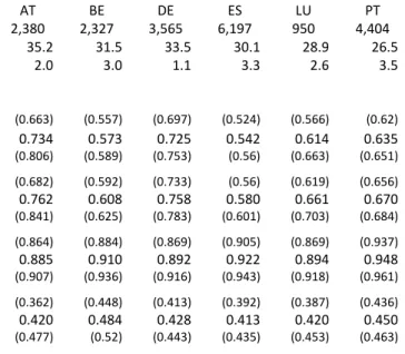
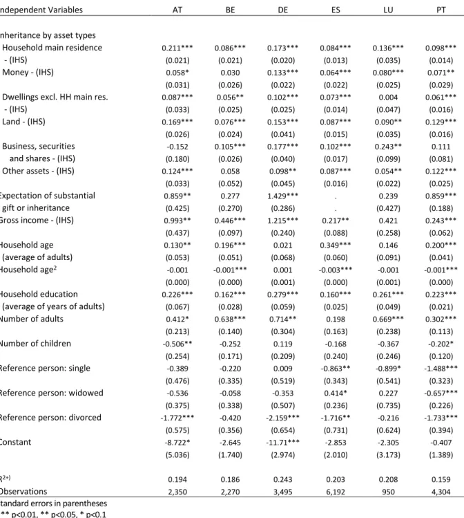
In a previous paper (Leitner, 2016) the Shapley value approach to decomposition was already applied on wealth inequality drawing on data from the first wave of the Household finance and consumption survey (HFCS 2010). Thus we can test the robustness of the results, comparing the outcome in the case of those countries that were analysed both in the previous paper and in this one. In the appendix we replicate the results of Leitner (2016) for those countries being analysed also in this paper (Austria, Belgium, Germany, Spain, Luxembourg and Portugal) for the decomposition of inequality in household net wealth. Comparing the figures in Table A.2 with our descriptive statistics based on HFCS 2014 in Table 1 above, we can see that most countries chose to increase the sample size, which should enhance the accuracy of the results. The share of households having inherited or received a substantial gift in
13
total households remains stable in all countries, except for Germany, where it fell from 34 per cent based on HFCS 2010 data to 27 per cent based on HFCS 2014 data. In the case of Portugal the share also declined somewhat, but only from 27 per cent to 23 per cent. Inequality in gross and net wealth holdings declined slightly from HFCS 2010 data to HFCS 2014 data in Austria, Belgium and Luxembourg, while in Portugal only in the case of gross wealth. In Germany and Spain there was almost no change in the Gini index of gross and net wealth. Particularly in the case of Austria the standard deviation of the estimated Gini indices fell both for gross and net household wealth indicating more accurate results. The Gini index describing household income inequality declined remarkably for Austria and Belgium, slightly for Portugal and increased somewhat for Germany and Spain. In order to understand the shift in income inequality a first consideration was, that changes in the survey methodology from the first to the second wave of the HFCS might have had an influence. In the case of Austria the interviewers used in the fieldwork of the HFCS 2014 new prefixed intervals in euro amounts to collect information on gross income (see Albacete et al., 2016). Looking into the HFCS 2014 dataset, we can see that the average income of the 10th decile surveyed is about 20 per cent lower compared to the upper decile in the HFCS 2010 resulting in a decline of the Gini coefficient describing income inequality from 0.42 (HFCS 2010) to 0.35 (HFCS 2014).
The regression results for the IHS transformed household net wealth based on HFCS 2014 data (see Table 2 above) remain very stable in comparison to the analysis performed with HFCS 2010 data (see Table A.3 in the appendix below). The coefficients are very similar for almost all inheritance asset types, education and household structure for most countries. In the case of household income a very strong increase of the coefficient can be observed for Austria, Belgium and Luxembourg, a somewhat lower rise for Spain and Portugal and a substantial decline for Germany.
Figure 3
Describing the changes between HFCS 2010 data and HFCS 2014 data for Austria, a similar picture can also be seen when drawing the unconditional relationships between gross income and net wealth. In Figure 3 we plot the percentiles of the IHS transformed data of the 2010 and 2014 waves of the survey.
-15 -10 -5 0 5 10 15 20 25
9,5 10,5 11,5 12,5
Net wealth -(IHS)
Gross income - (IHS)
HFCS 2010 HFCS 2014 Linear (HFCS 2010) Linear (HFCS 2014)
Source: HFCS 2010 - UDB 1.1, HFCS 2014 - UDB 2.0, wiiw calculations.
Scatter plot: Gross income versus Net wealth, HFCS Austria
percentiles of survey data - transformed by the inverse hyperbolic sine function (IHS)