An overview of the model for short-term forecasts

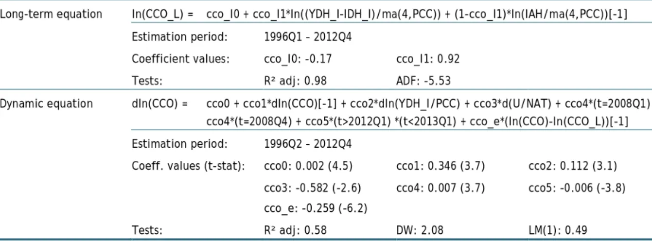
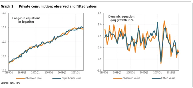
Compared to the 2003 version of the behavioral equations, empirical validation has been prioritized over theoretical priors. As in the previously published version of the model, household consumption9 is determined in the longer term by the real disposable income and financial wealth accumulated up to the previous quarter. As shown in Table 1, the ADF test clearly rejects the presence of a unit root in the residuals of the long-run equation.

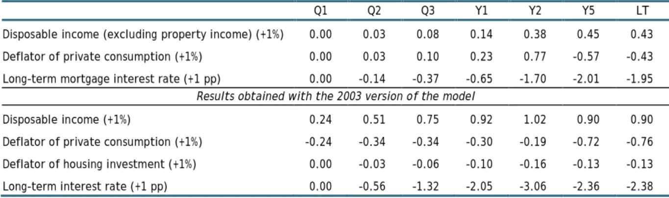
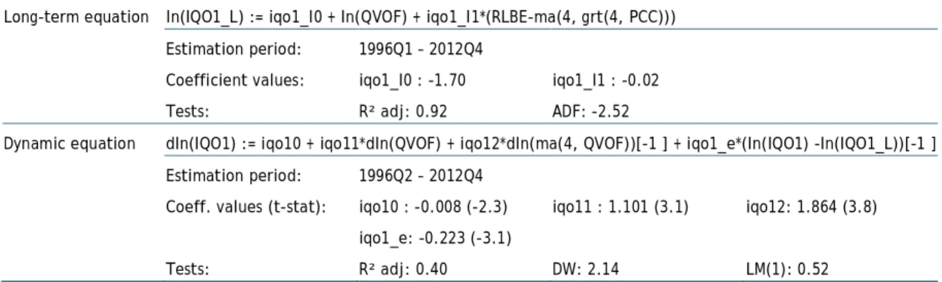
The income elasticity appears to be considerably smaller than in the 2003 version of the model. Most of the adjustment has taken place after two years, with an investment decrease of approximately 1.6%. Because the interest rate appears in the equation in logarithm, the semi-elasticity will vary depending on the initial level of the interest rate.

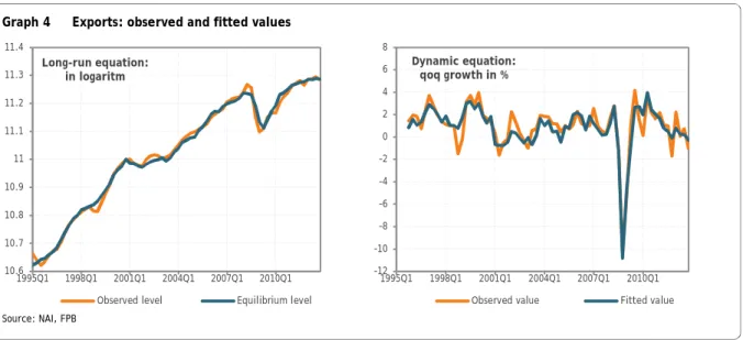
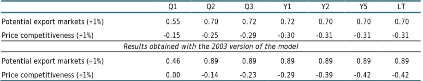
The long-term specification ultimately withheld is close to that in the version of the 200319 model, except that we have now omitted the trend responsible for the systematic loss of export market share since the late 1990s. As a result, the elasticity of potential export markets (0.70) is now smaller than in the 2003 version (0.89) of the model and an elasticity equal to one is statistically rejected. The low level of the LM test indicates the absence of first order autocorrelation in the residuals.

This rapid adjustment towards the long-term values ​​reflects the high value of the coefficient of the error correction mechanism, which is amplified by the autoregressive term.

Main deflators

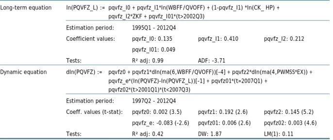
Both variables appear in the dynamic equation as a (lagged) moving average, indicating that they feed into prices only very gradually. All coefficients in the dynamic equation are significantly different from zero at the 5% level, while the Durbin-Watson and LM statistics confirm the absence of serial correlation in the residuals of the equation. The bump in simulated values ​​in the fourth quarter of 2002 is due to the dummy in the long run equation.

The right-hand panel shows that an important part of the short-term fluctuations remains unexplained, but that the main cycles in the growth rates of the deflator are well captured by the equation. After four quarters, only about 25% of the long-run effect of the determinants is visible in the deflator. All estimated coefficients in the dynamic equation are significantly different from zero at the 5% level.

On the other hand, the private value added deflator was not included in the dynamic equation in the 2003 version, whereas it now has a prominent role, even leading to an overshoot in the first years of the simulation. The tests point out that the residuals in the dynamic equation do not show serial correlation. The elasticities in Table 17 show that import prices are mainly determined by international non-energy prices, as in the 2003 version of the model.

In the longer term, underlying inflation adjusts to the long-term value of domestic prices and to import prices. 25 A Wald test clearly rejects the hypothesis that the coefficient for oil prices in the long-term equations for import and export prices of energy products is equal to one (see Appendix 1). In the short term, underlying inflation depends on developments in unit labor costs and import prices.

The LM test statistic shows that the absence of serial correlation in the residuals cannot be rejected. As can be seen in the right panel of Chart 9, the main accelerations and decelerations of underlying inflation are well captured by the equation, although much of the short-term volatility remains unexplained. Due to the small value of the error correction coefficient in the dynamic equation, this adjustment is very slow, reaching only about one-fourth of the long-term effect after two years.

The impact of a change in unit labor costs is temporary as it only appears in the dynamic equation. In the long run equation investment deflators are explained by (the long run value of) domestic prices and import prices excluding energy.

Wages and wage earning employment in the private sector Wages in the private sector

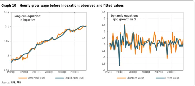
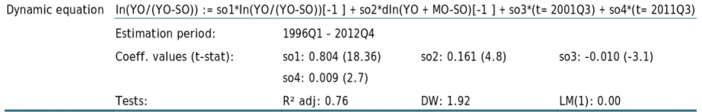
A permanent 1% hit to labor productivity translates into an increase in gross wages before indexation of 0.28% after one year and 0.48% in the long run. A one percentage point increase in the unemployment rate pushes wages down by 0.40% after one year and by 0.76% at steady state. As with business investment, wage employment in the private sector (expressed in total hours worked and excluding specific subsidized categories) no longer derives explicitly from a production function.

While in the 2003 version we assumed a Cobb-Douglas technology, this time we tested a more general functional form. However, decomposing productivity into labor efficiency and the real wage component turned out to be empirically impossible, because both components show a similar downward trend in the sample. Therefore, we decided, as an exception to the modeling strategy maintained for the other equations, to set an elasticity of 0.5 for real wages29 and of 1 for value added.

In order to account for the observed decline in productivity growth, a break in the linear trend was introduced in 2004. In the dynamic equation, the growth rate of both real wages and value added is highly significant. The dynamics along the cycle are also very well captured as can be seen in the right-hand panel.

According to the estimated equation, employment increases by 0.20% during the first quarter after a 1% shock to value added. The response to an increase in value added in the short term was quite similar to the 2003 version, but further adjustment to the long-term target was much slower.

Model simulations

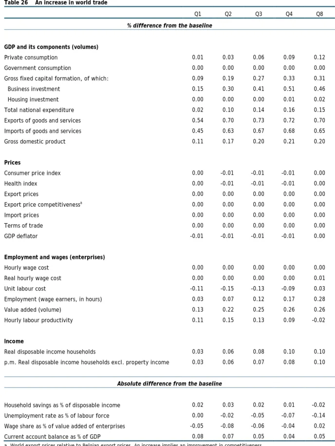
• An increase in world trade
• A euro depreciation
• A reduction in employers’ social security contributions
• An increase in the VAT rate on private consumption

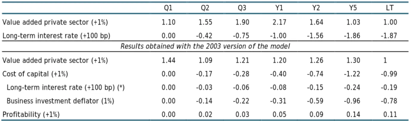
This increase in employment means higher disposable income, resulting in a modest increase in private consumption expenditures (+0.09% in the fourth quarter). A significant part of the increase in final demand is met by imports from abroad (+0.68% in the fourth quarter), since the elasticity of imports in relation to the reweighted indicator for final demand exceeds one. Furthermore, we assume an increase in Belgium's export market indicator (relative to its base level) of 1.5% in the first year and 2.3% in the second year, as Belgium's main trading partners are within the area of euros and enjoy better growth prospects thanks to an improvement in price competitiveness.

The improvement of economic activity and the built-in indexation mechanisms of some components of income gradually return real disposable income to the starting level in the second year. Competitiveness decreases slightly as Belgian export prices rise, bringing exports somewhat closer to baseline (from +2.34% in the sixth quarter to +2.29% in the eighth quarter). Export prices themselves are driven by steadily rising domestic prices, which are the result of higher nominal hourly costs that are not fully compensated by higher labor productivity.36 The GDP deflator exceeds the baseline by only 0.59% in the eighth quarter, a result of losses in conditions exchanges, as international prices have a greater impact on import prices than export prices.

Employment in the private sector exceeds the baseline level by 0.24% in the first quarter and by 0.68% at the end of the first year. At the end of the second year, employment in the private sector improved slightly (+0.78%). This, together with the deterioration of the terms of trade38, mitigates the initial loss of the share of wages.

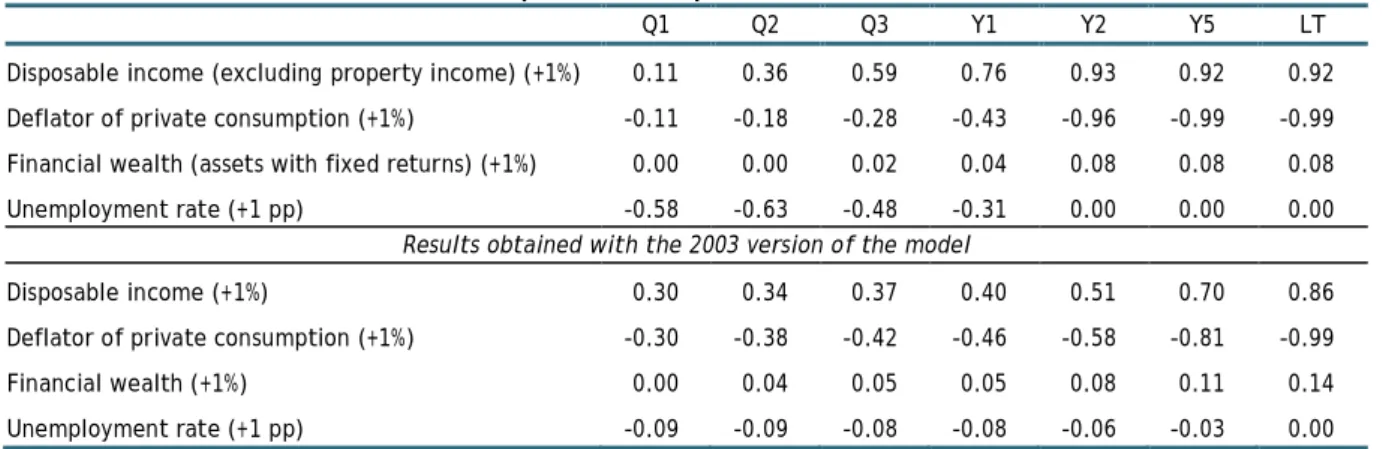
The deterioration of the current account balance reflects the conditions of trade losses and the increase in imports in volume. The impact of this measure on consumer price inflation is almost entirely concentrated in the first quarter (+0.86%). During the first year, private consumption (-0.17% in the fourth quarter) is less affected than real household disposable income (-0.23%), as a drop in the savings rate absorbs some of the the blow.

The loss in the total purchasing power of households is more limited in the second year (-0.10% in the last quarter) due to the recovery of income from real estate.41 However, private consumption remains significantly below its baseline level. (-0.35%). as it is mainly determined by real disposable income, excluding property income42 (-0.21% in the eighth quarter) and also because it is negatively affected by a rising unemployment rate. As a result, the savings rate rises above its baseline level in the second year. Then, employment worsens continuously (0.55% below the baseline in the eighth quarter) as a consequence of the decline in value added and the increase in real hourly wage costs43.

The decrease in domestic demand leads to lower imports, which, given almost unchanged exports and slightly improved terms of trade, implies an improvement in the current account balance. 41 This recovery is largely due to increased savings in the second year and the (purely technical) assumption that nominal long-term interest rates fully reflect the increase in inflation.

Coefficient restriction tests for level equations

Glossary