The NIME Model

The Federal Planning Bureau (BFPB) is a government agency under the authority of the Prime Minister and the Minister of Economic Affairs. So far, the Agency's efforts have led to the construction of a first version of the New International Model for Europe (NIME), the different parts of which will be presented in several working papers. The model describing the Belgian economy would consist of the short- or medium-term macroeconomic model currently in use at the Federal Planning Bureau.

We start by deriving the household sector's long-term equilibrium plans on the basis of an intertemporal optimization problem. The resulting set of demand equations explains the demand for goods, services and assets as a function of the nominal interest rate, the real interest rate, the user cost of residential buildings and the available funds. Finally, estimation results are shown for the household sector in the EU, NE, US and JP blocks.

I Introduction

In the second part of this article, we derive the long-term equilibrium plans of the household sector based on an intertemporal optimization problem. The resulting set of demand equations explains the demand for goods, services and assets as a function of the nominal interest rate, the real interest rate, the operating costs of residential buildings and the available resources. In the empirical part, we assume that rigidities prevent households from immediately adjusting their spending to their long-term equilibrium plans.

II Specification of a Set of Demand Equations for the Household Sector

The intertemporal allocation problem of the household sector

WHUt : total available funds of the household sector, in current prices, WRGt : wage in the public sector, in current prices,. In other words, equation (1) states that the total disposable assets of households are equal to the stock of assets inherited from the past plus the income generated by these assets and by the labor supply. The details of sources of labor income are used here for easy future reference when we present the Labor Market Analysis document in NIME.

Equation (8) describes the intertemporal utility function of the household sector, while equation (3.c) describes the intertemporal budget constraint. To hold one unit of real money balances, Mt/PCHt, one must spend PCHt units of the currency. The expected purchasing power in period t+1 of one purchased unit in period t is equal to (1+LICt)/PCHt+1.

A set of demand equations

In other words, system (14) determines the quantities demanded of a particular good as a function of available resources, the nominal interest rate, the cost of use of residential buildings and the real interest rate. When nominal interest rates rise, the opportunity cost of money will rise and the demand for money will fall. The impact on demand for other goods and services is a priori less clear; it is an empirical matter to determine the exact sign of the elasticity.

When the real interest rate rises, we expect that, ceteris paribus, the household sector will reduce its simultaneous consumption and save more by holding interest-bearing assets. An increase in the nominal interest rate increases the user cost of residential buildings, and will reduce the demand for residential buildings. It is not clear a priori how the change in user costs will affect the demand for consumer goods and the demand for money; they can be substitutes or complements.

III The Empirical Results

The data: sources and empirical regularities

Towards empirical application

The dynamics of expenditure on residential buildings is best captured by a partial adjustment scheme. We assume that rigidities exist that prevent the contemporary stock of residential buildings, CIROt, from immediately adjusting itself to the desired level. Equation (20) explains contemporary gross fixed capital formation as a function of the change in the desired capital stock, and the lagged gross fixed capital formation.

Here we assume that the long-term stock of residential buildings is described as1: (21) CIROLt = gir_l0 + gir_lb [DIHt / PCHt] + gir_l1 ln[USERIRt/PCHt]. Implicitly, we assume that the cross elasticities of the other prices are equal to zero. The long-run elasticities are obtained by evaluating equation (22) for GIROt = GIROt-1 = GIRO and DIHt = DIHt-1 = DIH.

First, it should be noted that the behavioral equations include the expected value of the future consumer price index, PCHt+1, and the expected value of the future price of housing, PCIRt+1. Second, all expenses in the empirical application are defined as expenses per capita, that is, we divide the expenses by the total population, NPO. Third, the interest rate LIC is a weighted average of the long-term interest rate and the short-term interest rate.

We insert the unit elasticity of scale in the short-run and long-run money demand equations. Sixth, we estimated the error correction mechanism using the two-stage Engle-Granger method (see Engle and Granger (1991)) and added some dummies to the equations. DUMGE is a dummy that captures the effect of German reunification, while UKBUILD is a dummy that captures the shift in UK monetary data caused by the inclusion of building society deposits in monetary aggregates since 1987.

The period up to 1981 was a period of high inflation and large inflationary differences between the countries of the EU and the NE bloc.

The empirical results

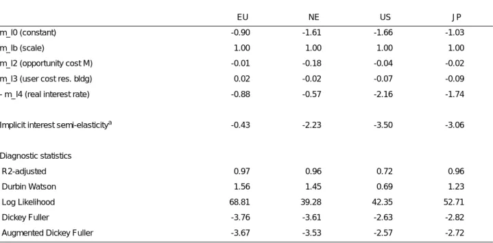
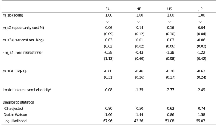
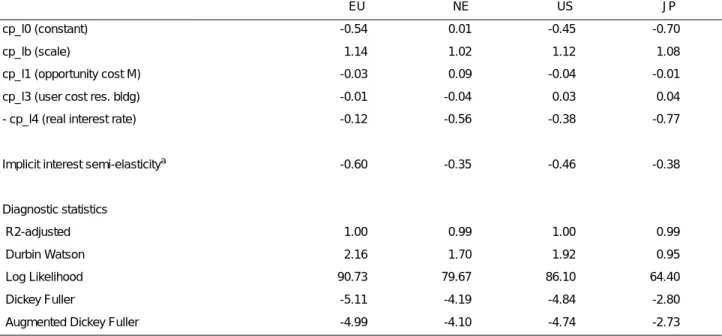
In most cases, the corrected R-squared is high, indicating that a fair amount of variation in the data has been accounted for. We obtain that for private consumption, long-run scale elasticities are greater than unity for all blocks, and larger than short-run scale elasticities. For example, the elasticity of real interest rates is negative in all equations of private consumption and money demand.

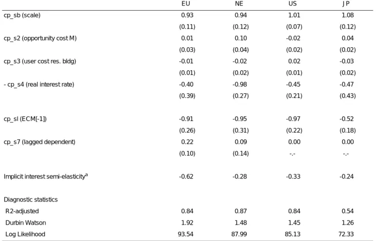
Finally, note that the sign of the user cost elasticity of residential buildings in private consumption and in the money demand function differs across countries. The rejection region of the null hypothesis is the region for which the DF test statistic without a cutoff is less than -1.99 (the test is inconclusive for values between -1.99 and -1.84) at the 5 percent confidence level, and the region for which the intercept DF test statistic is less than -2.33 (the test is inconclusive for values between -2.33 and -2.11) at the 5 percent confidence level. The "Semi-elasticity of implied interest" row measures the total impact of a change in the interest rate, as defined in equation (15.g).

Recall that interest rates affect demand through three channels: the liquidity effect, the intertemporal substitution effect, and the user cost effect. The numbers in this row summarize the total impact of a 100 point rate hike. We see that a rise in interest rates reduces the demand for goods, money and housing, both in the short and long term.

These results show, for example, that if the interest rate increases by 100 basis points, private consumption in the EU bloc will decrease by 0.6 percent, ceteris paribus. Likewise, we see a 0.5 percent drop in US private consumption when the US interest rate rises by 100 basis points. Point estimates for the formation of gross fixed capital of residential buildings show that in the short term there are significant differences in elasticity.

The high income elasticity of the US reflects the finding (see Appendix C) that the gross fixed capital formation series is a rather volatile one.

TABLE 1 - Long Run (Semi-)Elasticities for Private Consumption

IV Conclusion

V Appendix A: The Optimization Problem of the Household Sector

VI Appendix B: The Data

Household expenditure and revenue
Financial data
Missing observations
The definition of the aggregates of the country blocks

For blocs consisting of more than one country, a new monetary unit is defined. For the NE block, the unit is a weighted average of the currencies of Denmark, Greece, Sweden and the United Kingdom. XX_ZU: expenditure at current prices for Z in block XX, expressed in the currency of block XX.

PPP_XX_i: the purchasing power parity exchange rate, number of units of the currency of block XX, per unit of the currency of country i. XX_ZO: expenditure in constant prices for Z in block XX, denominated in the currency of block XX,. PPP_XX_i1990: the purchasing power parity exchange rate, number of units of the currency of block XX, per unit of the currency of country i.

VII Appendix C: Empirical Regularities of Some Key Variables

Trend Behaviour

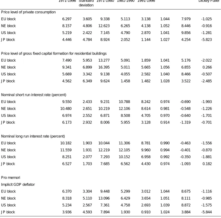
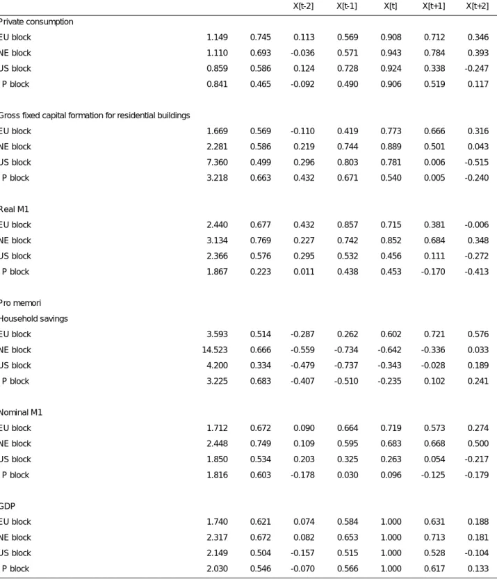
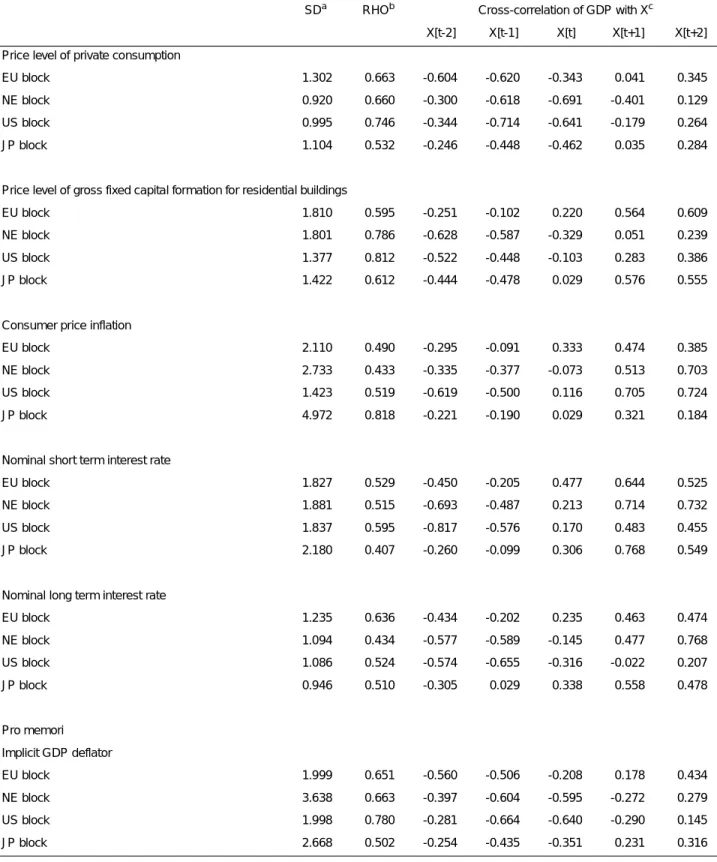
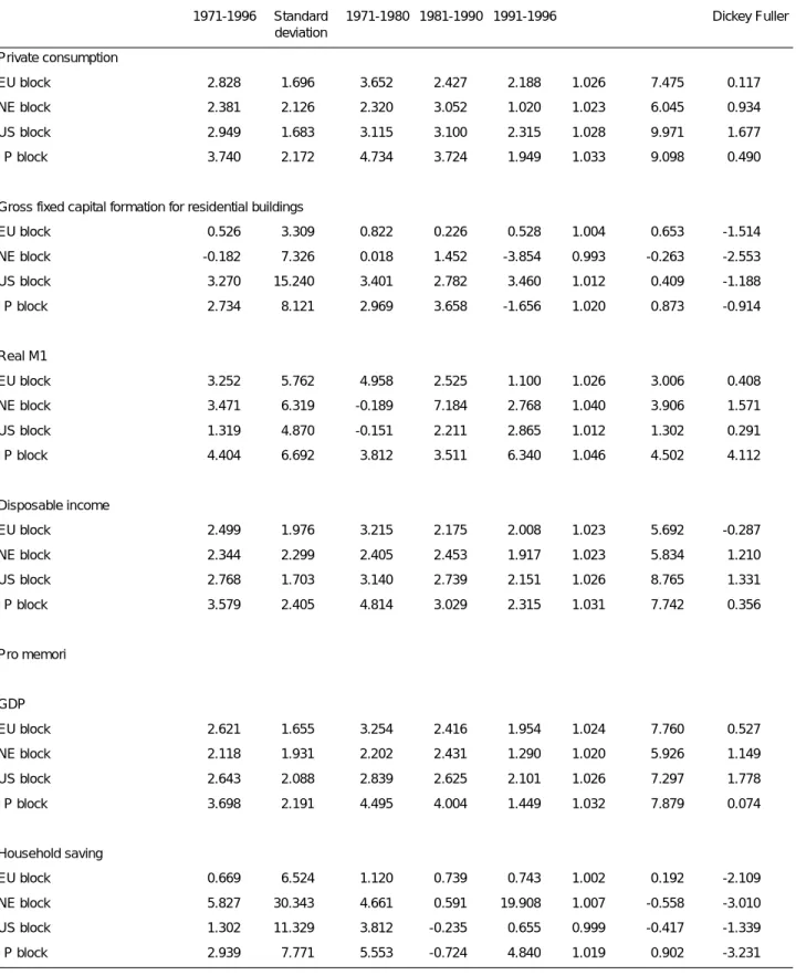
The second column shows the average growth rate of the variable over the entire sample period. The sixth column shows the autocorrelation coefficient RHO, while the seventh and eighth columns show the Dickey Fuller and Augmented Dickey Fuller test statistics, respectively1. The evidence in Table C2 indicates that the average growth rate of private consumption exceeded the average growth rate of GDP across all country blocs.

The average growth rate of gross fixed capital formation in residential construction was highest in the US and lowest in the NE bloc. This growth rate was even negative in the NE and JP blocks during the period 1991-1996. Of particular interest is the rather high standard deviation of gross capital formation growth in the United States.

The growth rates of real money balances vary quite strongly across blocs: decreasing in the EU bloc, starting from a negative average value in NE. The highest average price increases are recorded in the NE bloc and the lowest in Japan. Note that the NE block had the highest mean increase and the highest standard deviation of the GDP deflator, i.e. 8.3 percent and 5.1 percent, respectively.

Under the assumption that ut is white noise, one continues to estimate B in equation (C.2) and test H0 : B = 0, i.e. Lower and upper critical values are provided for the Dickey Fuller (DF) test statistic in, for example, Charemza and Deadman (1993). If the t-statistic is greater than the upper critical value, the null hypothesis cannot be rejected.

When this assumption is not met, the Augmented Dickey Fuller (ADF) test statistic is calculated, evaluating (C.3) d Xt = B Xt-1 + gk d Xt-k + ut.