First, for each country block there is a representative agent that captures the behavior of the entire business sector. Fourth, the natural rate of unemployment and the constant productivity growth of the factors of production are exogenous.
I Introduction
The starting point of the analysis is a sequential negotiation process in which, in the first stage, the utility-maximizing household sector and the profit-maximizing business sector negotiate the real wage. First, we determine the objective function of the various economic entities participating in this negotiation process.
II Equilibrium Factor Demand and
Factor Prices: Some Analytical Results
- The enterprise sector’s objective function
- The household sector’s objective function
- Factor demand
- The wage setting equation
- The price of the private capital good
- The price of imports
- The steady state
The weights depend on the relative bargaining power of the household sector and the business sector. Equation (17) says that the price of capital is equal to the discounted future - after taxation - market value of the marginal productivity of capital1.
III Factor Prices and Factor Demand
The Empirical Results
The price of labour
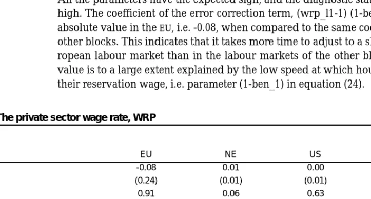
We assume that the reservation wage in the medium run is proportional to the net wage in the private sector. Equation (26.b) states that in the steady state the real wage is proportional to the marginal productivity of labour.
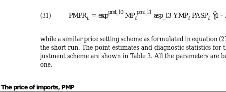
The price of capital and imports
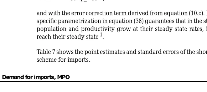
The Durbin h test statistic is calculated by adjusting the Durbin-Watson statistic for the fact that the equation includes a lagged dependent variable (see Johnston (1985)). The point estimates and diagnostic statistics for the short-term adjustment scheme are shown in Table 3.
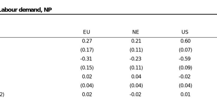
The empirical results for factor demand
We will now explain how this predetermined level of output, together with predetermined prices, determines factor demand in the short run. The empirical question is to determine the sign of the elasticity of the user cost of capital and the price of imports. However, it should be remembered that due to the Cobb-Douglas nature of the production function, the long-run output elasticity is 1, the long-run wage elasticity is -1, and the cross-price elasticities are equal. to 0.
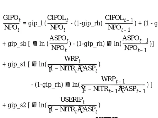
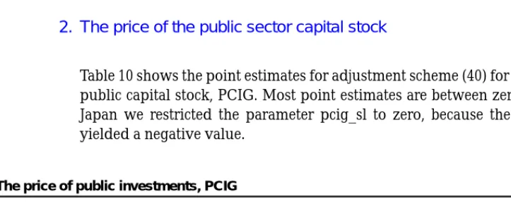
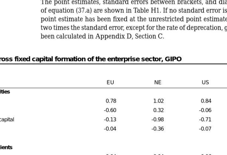
CIPOLt: the desired capital stock in period t, at constant prices, Xt: a short-term adjustment variable. For gip_l, the parameter that measures the speed of adjustment of the effective capital stock to its desired level, it follows that: 0 < gip_l < 1. Equation (37) explains the simultaneous gross fixed investment as a function of the change in the desired capital stock, lagged gross fixed capital formation and any other variable X that may affect adjustment in the short run.
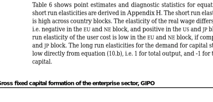
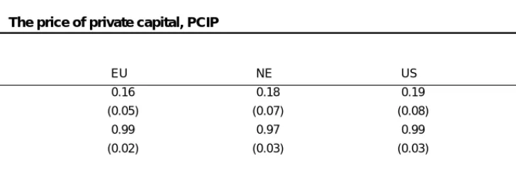
The short-term user cost elasticity is low in the EU and NE blocs, compared to the US. See equation (H.3) of Appendix H for the calculation of the short-run elasticities of gross fixed capital formation. Note the rather high values of the elasticities compared to the elasticities of the other factors of production.
IV The Prices for Final Users
The price of private consumption goods
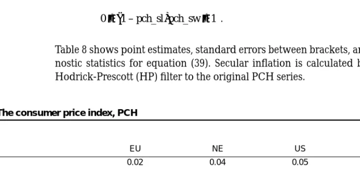
HP_ASPO: the stable supply of private demand from the private sector, PCH: the price of private consumption. Remember that the parameter px_sl measures the fraction of the composite price that is kept at its old price and that the parameter px_sw measures the fraction of the composite price that is revised according to a rule of thumb2. The parameter pch_s1 refers to the feedback of the output gap to the adjustment of the simultaneous price to its equilibrium value (see equation (F.13) in Appendix F).
Secular inflation is calculated by applying a Hodrick-Prescott (HP) filter to the original PCH series. All point estimates have the expected sign, but it should be noted that the value of pch_sl is quite low. We also show in this table the reduced form point estimates of the output gap, secular inflation and cost-push inflation.
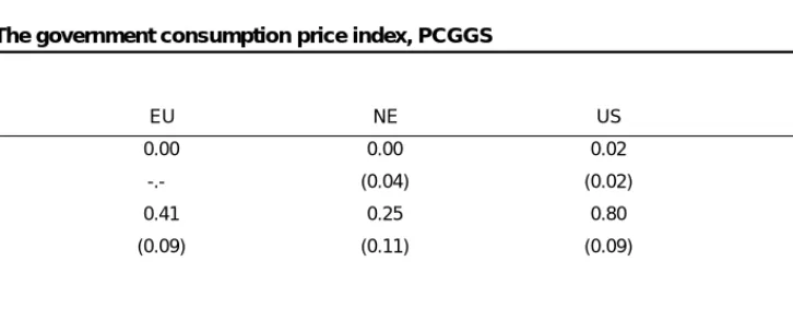
With G_PCHt = ln(HP_PCHt) - ln(HP_PCHt-1), where HP_PCH is the steady price of private consumption. In other words, (1-px_sw) measures the fraction of the price of public consumption that is revised to the "rational reset price".
The price of the other goods
The export of one block is the import of the other blocks, where they are used in the production process. EFEXt : the effective nominal exchange rate, amount of local currency per unit of foreign currency. EFYMPt: the productivity of imports in the production process of the rest of the world.
Here we see relatively higher values for pxt_sl, indicating that for exports the price remains unchanged for a longer period, compared to other prices. ASPOt: total supply for final demand from the enterprise sector, at constant prices, ASPUt: total supply for final demand from the enterprise sector, at current prices.
V Summary
We conclude the empirical section of the paper by showing the evaluation results for prices for end users. There, we once again showed that price revisions are generally not strongly constrained by menu costs, leading to relatively high values for the parameter of the error correction term.
VI Appendix A: The Optimization Problem of the Enterprise Sector
- The intertemporal optimization problem
- The user cost of capital
- The factor demand equations
- The unit cost function
- Constant returns to scale and profit maximization
- Gross fixed capital formation and the capital stock
Using this capital stock in period k will degrade its value by gip_rh percent, so that you get a price equivalent to selling the capital stock in period k+1. Equation (A.8.a) determines the equilibrium private supply price for final demand in terms of the costs of the factors of production. Constant return to scale and profit maximization. which can be rewritten assuming constant returns to scale as:.
VII Appendix B: The Wage Setting Equation
The bargaining process
Equation (B.7.a) states that the real wage is a weighted average of labor productivity and the reservation wage.
Derivation of the wage equation (7.a) and (7.b)
Using (B.10) and (B.11) and assuming constant returns to scale in the production process2, equation (B.9) can be rewritten as:
The bargaining power and the unemployment rate
VIII Appendix C: Some Steady State Properties of the NIME Model
- The natural level of employment
- The natural level of output and factor productivity
- Relative factor prices and relative factor productivity growth
- Real factor prices and productivity growth
- Output prices and productivity growth
Equation (C.10) defines the steady state level of output as a function of the natural level of employment, relative factor productivity and total factor productivity. Equation (C.12) sets a constraint on marginal productivity: the sum of the marginal productivities of the various factors of production must equal the total factor productivity. Let us now assume that in the steady state the relative factor prices do not change.
It should be noted that although relative factor prices do not change, real factor prices do change in relation to real productivity growth. It therefore follows that if we assume that factor prices grow at the same rate2, and that net indirect taxes remain unchanged, then the price of aggregate supply also remains unchanged.
IX Appendix D: The Data
- Private supply for final demand
- Private sector employment
- The capital stock of the enterprise sector
- The user cost of capital
- The consolidated imports of the EU and NE blocks
XX_GDPO: gross domestic product of block XX, in constant prices, XX_MTO: consolidated imports of block XX, in constant prices, XX_WBGO: the wage bill of the government, in constant prices,. The latter is equal to the operating surplus of the household sector, corrected for household consumption of residential buildings. XX_CIPU: stock of fixed capital held by the private sector of block XX, in current prices,.
XX_DEPPU: consumption of fixed capital of the private sector of block XX, at current prices. XX_GIPU: the formation of gross fixed capital from the private sector of block XX, at current prices. Equation (D.4) states that the stock of private capital in period t depends on the stock of private capital in period t-1, and the net investment flow in period t.
The rate of depreciation of the private capital stock, gip_rh, is calculated as the average ratio of , calculated over the period. Implicitly, we assume here that the business sector's operating profit accrues to capital. The import data for the EU and NE blocs must take into account that trade between countries in the same bloc cancels out at the bloc level.
X Appendix E: The Wage Dynamics
XI Appendix F: The Price Dynamics
- The assumptions
- The “rational” reset price, PXR
- The “rule of thumb” reset price, PXB
- An adjustment scheme
We will now specify the "rational" reset price and the "rule of thumb" reset price. The relationship between the producer price and the price paid by the end users is described in equation (40.b) of the main text. Therefore, if one wants to calculate the price of total supply for final demand, one must calculate all the cost components listed on the right-hand side of equation (F.3).
Second, the following assumptions are made regarding the observation of the various cost components given in equation (F.4). Equation (F.6) states that the "rule of thumb" reset price, PXB for X = CGGS, CIR, CIG, is equal to the lagged price, plus the change in indirect taxes, plus the weighted average of the change in the lagged price and the change in the contemporaneous import price. In this section, we provide an equation for the short-term price determination based on the equations derived in the previous sections.
Equation (F.10) explains the change in PX with an error-correction term, a term that measures the contemporaneous change in marginal costs (ie the restored rational price), a partial adjustment term, and the lagged cost push inflation. We will deal with this problem in the next sub-section, starting from the assumption that the price of private consumption clears the goods market. We will now make the following assumptions about the variables on the right side of the equation (P.12).
XII Appendix G: An Error Correction Mechanism for Labour and Imports
- The short run factor demand equations
- Factor demand and steady state growth
- The error correction mechanism of labour demand
- NITR )
However, if we want employment and imports to be consistent with sustainable population and productivity growth, then we must impose the following additional constraints. In other words, condition (G.12) is a constraint on the parameters that must be satisfied if one wants the steady state to be reached when productivity increases at its steady state rate. Note also that in the steady state, the second part of the error correction term is equal to HP_NP.
Equation (G.23) states that concurrent employment deviates from its natural rate to the extent that output deviates from its natural level, and that the real wage deviates from marginal productivity.
XIII Appendix H: A Partial Adjustment Scheme for Gross Fixed Capital
This implies that the short-run elasticity of output, ASPO, is equal to1: (H.3.a) cip_l1 + cip_sb. The point estimates, standard errors in parentheses and diagnostic statistics of equation (37.a) are shown in Table H1. If no standard error is shown, the point estimate is fixed at the unconstrained point estimate plus (or minus) twice the standard error, except for the rate of depreciation, gip_rh, calculated in Appendix D, Section C.
XIV References