In this work, a noise prediction framework based on the Blade Element Momentum method for aerodynamic prediction was coupled to the empirical aeroacoustic models based on the works of Carolus et al (2007) and Brooks et al (1989) and to XFOIL for boundary layer parameters . calculations. A parametric study was conducted to determine the impact of fan diameter and number of blades on the noise produced.
Nomenclature
G1 Peak level function for TEB-VS noise G2 Spectral shape function for TEB-VS noise G3,G5 Spectral shape functions for LBL-VS noise G4 Peak level shape function for LBL-VS noise h Sharpness thickness of the back end. Naz Number of azimuthal divisions NB Number of fan control point blades Pi B'ezier.
Introduction
- Air Conditioning Worldwide
- Environmental Impact of Air Conditioning
- Noise Legislation
- Objectives
- Thesis Outline
Therefore, these figures can be used as a first-order indicator of the energy demand for both cases. Chapter 3 describes the properties and operating principles of the custom aeroacoustic tool that will be used.
![Figure 1.1: Schematics of an outdoor AC unit [2].](https://thumb-eu.123doks.com/thumbv2/123dok_br/19768390.0/22.892.233.664.105.460/figure-1-1-schematics-outdoor-ac-unit-2.webp)
Fan Aeroacoustics
Sound and Noise
Sound Pressure Level and Noise Scales
In order to assess typical values in this scale, the sound pressure levels for some example sounds are shown in table 2.1. The sound pressure level objectively quantifies the intensity of a sound, but it does not take into account the effect of sound frequency in its perception by the human ear.
Tonal and Broadband Noise
The relationship between sound frequency and loudness change is shown in Figure 2.1. In fact, all the sounds we know are a complex combination of sound components of different frequencies and intensities that make up the so-called sound spectrum.
Fan Noise Mechanisms
- Mechanical Noise
- Aeroacoustic Noise
In a manner similar to trailing edge blunting noise, tip vorticity noise is the result of vortices shedding at the blade tip due to the pressure difference between the top and bottom surfaces. Although it is broadband noise, there is a relationship between the frequency of the noise produced and the size of the eddies.
![Figure 2.2: Frequency spectrum of a sound [11].](https://thumb-eu.123doks.com/thumbv2/123dok_br/19768390.0/30.892.211.687.109.421/figure-2-2-frequency-spectrum-of-sound-11.webp)
Noise Prediction Method
- TEB-VS Noise Prediction Model
- Tip Vortex Formation Noise Prediction Model
- LBL-VS Noise Prediction Model
- TBL-TE Noise Prediction Model
- Turbulent Inflow Noise Prediction Model
- TBL and TE Alternative Models
- Directivity Functions
- Boundary Layer Parameters
The function G1 determines the highest level of the spectrum and is a function of the thickness ratio. The coordinates ξ1 and ξ3 are part of the rotating reference system defined in the model shown in Figure 2.10, together with the stationary coordinate system used. Therefore, the noise prediction method in this work is supplemented by an external calculation of the boundary layer parameters using the XFOIL code [26] or the RFOIL code [27].
![Figure 2.9: Variables used in tip vortex noise prediction [15].](https://thumb-eu.123doks.com/thumbv2/123dok_br/19768390.0/38.892.280.631.109.456/figure-variables-used-tip-vortex-noise-prediction-15.webp)
Blade Element Momentum Theory
- BEM Corrections
- Fan Efficiency
A drawback when using XFOIL is that the code does not calculate the boundary layer thickness δ, necessitating the use of the relation given by Drela and Giles [28]. The quality of the results produced by the BEM method is very sensitive to the quality of the input aerodynamic data. Since the volumetric flow can be given by AV, the power of the flow delivered by the ventilator is given by.

Aeroacoustic Tool
Brief Description
The rotor input file is a text file that contains all the relevant parameters to define the fan geometry to be analyzed, such as the hub and maximum radius, the number of blades, and the sections that define the blade radially, among others. The analysis input file specifies all the analysis conditions, for example the number of radial elements on which the noise calculations will be performed and the corresponding noise models to be used or the physical constants that relate to the circumstances of the situation to be analyzed , such as air density, speed of sound, or mean inflow velocity. After the analysis is complete, the code can output all the results of the BEM calculations, such as the radial distribution of the angle of incidence, local Reynolds, relative velocities, etc.
Adaptation for a Low Speed Fan Case
Figure 3.1 shows a diagram of the relationship between code modules, libraries and external software they depend on, and inputs. Therefore, the basic equations of the BEM theory originally applied to the aeroacoustic vehicle had to be modified to reflect the operation of an axial fan, in relation to that presented in Section 2.6. The tool uses a turbulent input noise model of an atmospheric nature, due to the height of the wind turbine tower, which does not apply to the case study, since axial flow fans are usually enclosed in duct-type housings or in enclosed spaces, where wind turbulence is not present.
Validation
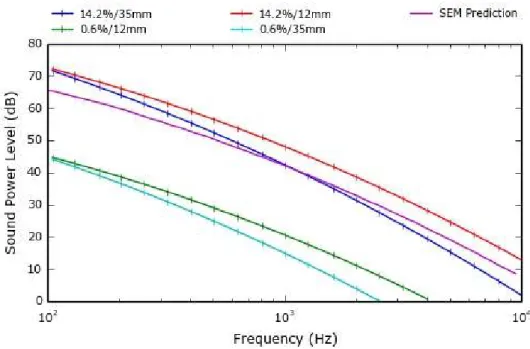
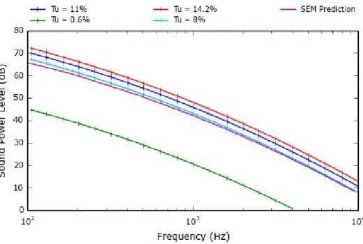
- Turbulent Inflow Numerical Model Validation
- Overall Spectrum Validation
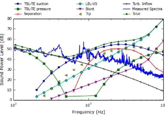
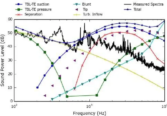
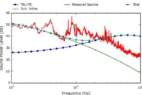
The total sound power spectrum of the fan, calculated by the tool, is shown in Figure 3.7, together with the contribution of each of the different noise mechanisms introduced in the tool. It can be seen that the results in the high frequency range have improved, but there is still an overestimation of the noise, with differences of 10 to 20 dB. The results are significantly better, such that the model underpredicts noise in the mid-frequency range, but overpredicts it in the high-frequency range.
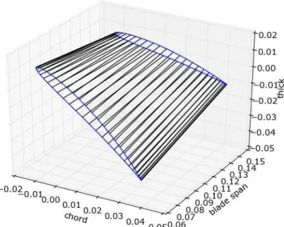
![Figure 3.2: Radial distribution of section geometry of fan used for validation [21].](https://thumb-eu.123doks.com/thumbv2/123dok_br/19768390.0/54.892.262.626.128.554/figure-radial-distribution-section-geometry-fan-used-validation.webp)
Blade Parametrization
Airfoil Description
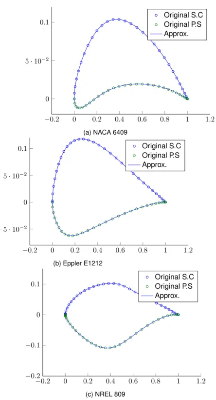
This fit was unsuccessful as shown in Figure 4.3 as the leading and trailing edges do not connect possibly due to the low order of the curves and the high curvature of the trailing edge of the pressure section. In addition, an algorithm resulting from the work developed in [45] was used to improve the results. Also in this algorithm, the formulation presented in equation (4.1) is transformed into an equivalent matrix formulation, where the coefficients of Bernstein polynomials, control points and various variables are t2, t3.
![Figure 4.1: Design variables defined in [41], [42] and [43].](https://thumb-eu.123doks.com/thumbv2/123dok_br/19768390.0/62.892.237.650.104.433/figure-4-design-variables-defined-41-42-43.webp)
4.2 3D Parametrization
This algorithm considers the "bending" of the input data set to arrive at a set of control points that produce a curve that goes "through" the given points, rather than just minimizing the mean distance between the approximation and the input data. Obtain the radial distribution of blade airfoil shapes, with all airfoils having a uniform chord; The advantage of this approach is that airfoil locations, twist distribution, and chords are independent of each other, allowing them to be optimized separately to examine the effect of each variable on the final results.
Baseline Fan Characterization
Blade Definition
In this way, if e.g. a 2ndorder B'ezier curve has a satisfactory fit, only 3 control points, or 3 airfoils in this case, are needed to describe the distance between the blade edges. Before the extraction of the airfoil sections, the leading edge of the blade had to be modified by rounding it with a radius of 0.1 mm. With all the geometric parameters defined and introduced in the code, the final blade geometry was produced by the program.

Aeroacoustic Analysis
In this case, these points are calculated and extracted from the model for each section. With this new geometry, the required polars were calculated and entered into the code and the analysis was run. The two models mentioned in chapter 3 were used in two different analyzes to choose which one produces the results closest to the experimental data.

Experimental Correlation
Since the value of the difference is similar in both cases, the criteria to choose the method should be the predicted OASPL and it should be compared with the experimental one. Although the discrepancy in the low frequency zone is acceptable, the correlation in the remaining spectrum is not satisfactory, with differences of the order of 20 dB(A) between the predicted and the experimental results. In table 5.5, the values of OASPL obtained by the two variations of the first method and the second method are presented, together with the error compared to the OASPL provided by the air conditioner manufacturer of 61.4 dB(A).

Geometrical Parametric Study
Fan Diameter
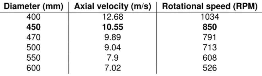
Since the number of leaves in the present case remains the same, equation (6.3) reduces to. Using the expressions presented, the rotational velocities and axial velocities used in the analysis for each diameter value were obtained and are presented in Table 6.1. After entering these parameters and making the necessary geometric changes in the aeroacoustic tool, the noise predictions were obtained and are shown in Table 6.2.
Blade Number
Similar to the effect of increasing diameter, increasing blade number reduces the noise produced, although the magnitude of the reduction is lower than that observed when increasing diameter. When we compare the noise spectra, it can be observed that the peak observed around 3000 Hz remains relatively unchanged, except for the 3-blade case. This can be explained by following the same reasoning presented in section 6.1, since only the number of blades is changed, therefore the characteristic dimensions of the fan are unchanged and the frequency where the peak occurs is the same.

Fan Diameter and Blade Number
These deviations can be explained by the decrease in the rotational speed and chord when the number of blades increases and by the decrease in the axial flow velocity when the diameter increases, because lower chords and lower speeds lead to faster reaching of stall, which brings inaccuracy in the calculations. . From equation (2.59), it can be seen that as the rotational speed and the cord decrease, while maintaining the axial flow rate, the inlet angle must decrease so that the torque increases. It can be seen that this reduces the thrust produced, by inspecting equation (2.58), which in turn reduces the efficiency, at constant power and axial flow rate (see equation (2.70)).

Aeroacoustic Fan Optimization
Numerical Optimization Techniques
Once the function is defined, the optimization problem can be initialized by naming the design variables and defining their constraints. In [37], the effect of population size on convergence and running time was studied. As expected, as the population size increases, the number of generations required to reach convergence decreases, but the number of function calls required increases.
Problem Definition
Convergence of the solution One of the input parameters in an optimization using genetic algorithms is the size of the population created in each generation. These two parameters affect the convergence of the solution, because if they are too low, the solution may not converge and there is still more leeway in the design space to reach a better solution. Since the basis of the work that led to this conclusion is similar to the basis of this work, this rule will also be applied in the subsequent optimizations.
Optimization Cases
- Baseline Fan
- Improved Fan
When optimizing for the efficiency objective function, the obtained results showed an increase of 2.3% to 24.5%, with the convergence study presented in Figure 7.9. Optimizing the twist of the two objective functions, OASPL and Efficiency, the optimizer created the Pareto front shown in Figure 7.11. Since the compromise solution is similar to the maximum efficiency solution as shown in Figure 7.11, it was expected that the twist distribution was also similar, as a sudden increase in twist was observed in the tip region.

Conclusions
Achievements
In both cases, the combination of design variables that produce these results is the blade chord and twist. When comparing the new fan to the baseline fan, a total reduction of 17.5% in the OASPL is achieved, but at the cost of lowering the efficiency by 18.1%. With computational advances, the emphasis on improving the efficiency of the preliminary design stage of most engineering projects has increased.
Future Work
Given the conclusions drawn in this work, the most realistic approach to obtaining the best trade-off solution would be to increase the diameter to 550 mm, maintain the number of blades and change the chord and twist to a to achieve an optimal solution. This is why this tool is valuable, because it allows, with little computational effort, to analyze and optimize any preliminary design of an axial fan to improve its performance as much as possible.
Bibliography
Evaluation of the maneuvering coefficients of a self-propelled ship using a propeller model with blade element momentum coupled to a Reynolds averaged Navierstokes flow solver. Improved non-dominated genetic sorting algorithm (nsga)-ii in multi-objective optimization studies of wind turbine blades.
Appendix A
Noise Prediction Models Equations
TEB-VS
LBL-VS
TBL-TE
Appendix B
Coordinate Systems
![Table 1.1: Comparison between cooling degree days (CDD) and heating degree days (HDD) in the 50 largest metropolitan areas in the world [5].](https://thumb-eu.123doks.com/thumbv2/123dok_br/19768390.0/24.892.234.659.217.987/table-comparison-cooling-degree-heating-degree-largest-metropolitan.webp)
![Figure 2.10: Coordinate systems and variables used in the prediction of Turbulent Inflow noise [21].](https://thumb-eu.123doks.com/thumbv2/123dok_br/19768390.0/41.892.247.642.112.350/figure-coordinate-systems-variables-prediction-turbulent-inflow-noise.webp)