AERODYNAMIC OPTIMISATION OF A CONSTRAINED AEROFOIL’S SHAPE COUPLED WITH AN OPTIMISATION OF

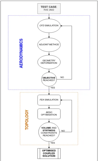
The overall aim of the work lies in the coupling of two optimization procedures for the main fields of study, the aerodynamics and the topology layout, by means of different open source resources, respectively SU2 and Calculix, which are able to provide robust and efficient simulations in both. studied directions. A migration procedure of the acquired data was required by the topology analysis of the aerodynamic output to apply the pressure loads on the airfoil surface as concentrated loads.

Glossary

SA Spalart-Allmara's model is a one-equation model which solves a modeled transport equation using the kinematic viscosity. The SIMP Solid Isotropic Material with Penalization method is a procedure used to predict an optimal material layout given a design space, loading, manufacturing, and boundary constraints and performance requirements using a constrained density-based study.

Introduction

Topic Overview

Another technique, the gradient-free method, faces the negative property of gradient-based procedures in some cases. An overview of the actual processes and applications is collected in the work done by Ji-Hong Zhu et al.

Motivation and Goals

Thesis Outline

Theoretical notes

Aerodynamics

• Reynolds Averaged Navier-Stokes equations
• Spalart-Allmaras turbulence model

The left side of the equation represents the transport model for the eddy viscosity and must be equal to the production term, followed by the diffusion term and ending with the destruction term. The velocity of a point inside the boundary layer for turbulent flow is proportional to the logarithmic value of the distance between the specified point and the nearest point in the wall [36].

Near-wall treatment

Laminar region and trip term

Sensitivity analysis

The problematic arises when trying to calculate the term involving the gradient of the variables from the actual solution (u) of the flow with respect to the design variables (D), ∂u/∂D in equation (2.30) . 2.37) If this is embedded in the final form of the sensitivity formulation (or total derivative), the final form is:.

Parametrisation techniques

Note that the adjoint solution depends only on the objective function L and not on the design parametersD and that there is an adjoint solution for every objective function defined. By manipulating the latest equation, a linear system is obtained whose complexity depends on the number of design variables:

Free-Form Deformation box

Mesh deformation

In [51], one of the forerunners for the mesh deformation algorithms, the authors recommended to provide a control in the manufactured deformations by following 3 steps. Furthermore, those eigenvalues ​​are also used to control the mesh quality, thus the second phase of the deformation study.

Structures

• Elastic behaviour of the model

The next step is to find the relationship between the six independent tensions and the nine independent components of the movement,²kl. Then, to begin with, the Cauchy stress is directly related to the strain gradient and the latter should not be expressed depending on the coordinates. The volumetric deformation can be expressed by the trace of the strain tensor, while the deviatoric strain tensor is obtained by using the general strain tensor and the volumetric strain tensor as below: 2.55) In view of a direct relationship between the elastic modulus E and the strain definition, the bulk modulus K and the shear modulus Ga are used.

Since the Lamé constants are not given for every material, equation (2.56) can be arranged using

2.2.2 (B)ESO methodology

Evolutionary Structural Optimisation

Then this cycle of element removal is performed using the same rejection ratio until a convergent condition is found, which in other words tends to say that no other cells are inefficient and the remaining ones are critical for the geometry's well-behavior. An example of the ESO procedure can be found in figure (2.5), where an optimal solution is given for a square hanging object under its own weight.

Bi-directional Evolutionary Structural Optimisation

This feature occurs when the model is discretized and compliance constraint minimization is applied. First, the volume strain energy is minimized, so the compliance parameter follows. This is when the filter should be applied using the nodal sensitivity of the node.

To take advantage of the method, the minimum row must be higher than half the element length.

CFD Methodology

• Case study introduction
• Mesh generation
• Approach towards the simulation
• Mesh convergence study
• Free-Form Deformation box
• Adjoint methodology

All these functions are defined by the user, and therefore the generation can be adapted to the goals of the project. It can be clearly seen which areas of the domain are more important and how small the cells are in the subregion of the boundary layer. Furthermore, one can notice that outside the boundary layer area the network is unstructured.

That way, the deformation of the CP would have more influence on the geometry closer to it.

Structural methodology

Case study

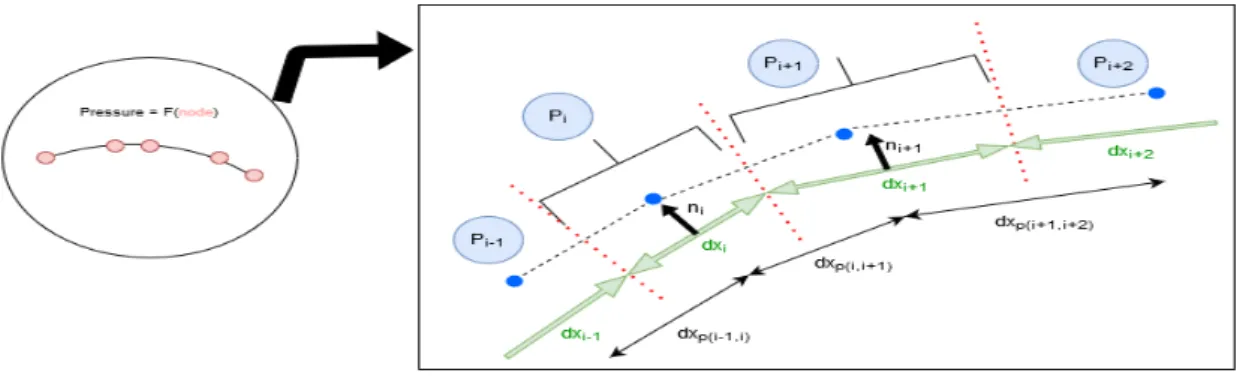
In most cases, this depends on the networking software and methodology used. From this point it was clear that the methodology must retain the nodal character of the CFD output, but a change in the pressure value must be made. The reason for this is a decrease in the speed of the flow and thus an increase in the magnitude of the pressure.

Once the migration procedure of the surface pressure from the CFD environment to the FEM is done, the implementation of the Calculix script must be defined.

Verification of the structural mesh

Moreover, all the loads follow each of the normal vectors obtained by the discretization procedure illustrated in Figure (4.2) and how the lower surface sizes are higher than the upper ones, leading to an upward lift force. To do so, the physical groups must be defined earlier in Gmshenvironment and then export the mesh file as the specified format. By doing so, it is simpler and easier to define the boundary conditions and constraints of the setup.

The constraints of the model were applied to the wing box, forcing zero displacements at its internal planes as can be seen in green in Figure (4.4), apart from the thickness-related threshold of 0.008c previously specified for the topology optimization process.

BESO procedure and the selected variables

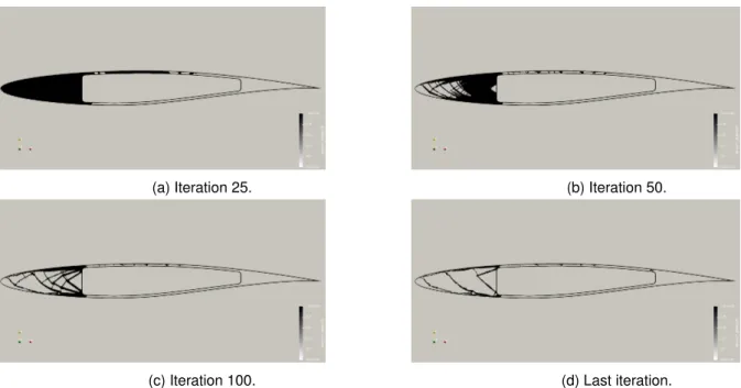
Expand sensitivity Element density takes maximum density in surrounding nodes. From this point and by examining the images, the effect of the filter can be understood. Note that the value shown in the mass size graph is a representative value of the amount of airfoil remaining area1.

For the highest removal ratio, figure (4.12), FI is twice higher than the yield stress parameter of the polypropylene material (σP Pyi el d=35MPa).

CFD Results

Flow simulation

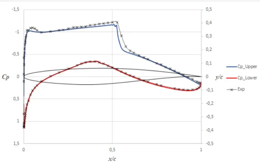
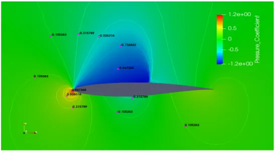
It is possible to see the similarity between results and where the shock wave appears, which is approximately at the x-axis position of 0.55c. From the last figures regarding the pressure coefficient and the Mach number distribution, it is possible to note where the shock wave appears and how it changes the behavior. This shock wave position slows the flow to values ​​below Mach 1 and subsequently, since the pressure gradient from the airfoil geometry is positive, the speed of the flow is further reduced.

Focusing in the trailing edge region, the boundary layer thickness grows with the positive pressure gradient provided by the geometry, but at the final vertex the upper and lower flows tend to be driven in the same direction.

Optimised aerofoil’s shape

On the other hand, the geometric changes at the leading edge, Figure (5.12a) in blue, increased, while maintaining the conditionality of the shock wave phenomenon with a decrease in velocity in this subregion. Therefore, in order to mitigate the interaction between the airfoil geometry and the airflow, the optimization algorithm performs a readjustment of the initial contact conditions in the leading edge, which is clearly visible in Figure (5.12a). As for the pressure coefficient distribution, Fig. (5.13), along the airfoil, the higher suction peak is closer to the leading edge than in Fig. (5.6), and the position of the shock wave has not been practically changed, although it is softened.

The results shown in Figure (5.16) follow the same trend as in the work done by Economon et al.

Structural results

Results

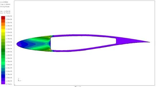
Therefore, most of the airfoil faces a higher structural demand due to pressure distribution. Moreover, the obtained quantities are lower than the elastic failure parameters of the selected material (aluminum allows 6061σyi el d=276M Pa). Nevertheless, the magnitude of the displacement is small (~10 µc) and will not have a direct influence on the aerodynamic behavior.

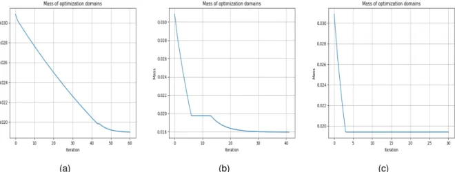
Figure (6.3) shows the path followed by the solver to achieve the optimization specific weight objectives.

Coupling between the optimised designs

Therefore, as in the development followed above, a comparison of the loads obtained by the nodal pressure for the general case and the optimized one is in Figure (7.7), and subsequently its structural analysis is presented. Since the initial setup is different from the general case study of the thesis, the expected behavior should be a variant. It is worth noting how very small changes in the aerofoil surface when optimizing the geometry have a large influence on the stress distribution.

With regard to the optimal reduction target, following the same explanation for the optimization of the general case study, the 25% target appears to be sufficient.

Conclusions and Future Work

Concluding remarks

The initial idea for the scope of the thesis was a general optimization coupling strategy, but the complexity involved required a lot of time and resources. Therefore, this tool can be considered very powerful, not because of the numerical and computational resources, but because of the free-choice design it offers. From the analyzed mass limits for material removal, using aluminum 6061T, a higher material reduction reached 10% of the initial mass, although its final geometric result appeared weak.

From this point, the study showed that the topology optimization process, in order to remove unnecessary mass, redistributes the internal stresses of the initial loaded airfoil towards the creation of rod structures, while reducing the maximum size shown in the non-optimized case, as the layout itself finds a more balanced state.

Recommendations and Future Work

At the end of the day, the software used gives an idea of ​​the path to follow in order to achieve specific optimization goals, but, as stated in the thesis, further post-processing needs to be done. For example, when an aerodynamic shape is optimized, it is only for certain flight conditions, so it does not consider the entire flight envelope. Therefore, the technique described in this thesis could, for example, be used to design the range of modifications that a variable geometry airfoil would need to make along the flight situation to be effective at all stages.

In addition to the aerodynamic point of view, several topology setups should be analyzed for the structural compliance in the situations described above and, as demonstrated in the thesis, if the mesh roughness gives specific elements higher stresses than those they realistically support, improved outputs can be achieved by using finer meshes and/or continuing to perform topology optimizations after the previously optimized solution has been subjected to a new geometry redesign with respect to the optimized case.

Jameson, "Studies of Continuous and Discrete Adjoint Approaches to Automatic Aerodynamic Shape Viscous Optimization," 15th AIAA Computational Fluid Dynamics Conference, 2001. Jameson, "A Comparison of Continuous and Discrete Adjoint Approaches to Automatic Aerodynamic Optimization ." 38th Aerospace Sciences Meeting and Exposition, 2000. Coles, “The wake law in the turbulent boundary layer,” Journal of Fluid Mechanics, vol.

Slater, “The Validation Archive of the NPARC Alliance, AIAA 99-0747”, in de 37e AIAA Aerospace Sciences Meeting and Exhibit, 1999.

Appendix A

Matlab ® script used to connect SU2 with Calculix

94% SAVE pressure loads for each of the nodes from the classified data 95 pvalue_UP = upperData(:,16);. 287 % AEROFOIL SKIN for topology optimization BOUNDARY CONSTRAINT ::> 2 mm 288 % WING−BOX SKIN for topology optimization BOUNDARY CONSTRAINT ::> 2 mm 289. 295 % REOPEN GMSH GEOMETRIC INPUT FILE TO PRINT 2 fo96' file. SurfaceTOGeoFile.txt','w');.