Coupled Preliminary Design and Trajectory Optimization of Rockets using a Multidisciplinary Approach

Neste trabalho foi criada uma ferramenta para otimizar o projeto preliminar de um foguete. A otimização do projeto é realizada por meio de um algoritmo genético contínuo desenvolvido e testado no trabalho, com opção de processamento paralelo.

Nomenclature

Acronyms

Introduction

• Motivation
• Rocket Design Challenges
• Rocket Design and Optimization
• Objectives and Deliverables
• Thesis Outline

The optimal launcher is selected by evaluating the performance and cost of the alternative designs. The use of approximation models is sufficient to correctly estimate the design characteristics of the vehicle [23].

Rocket Fundamentals

• Rocket Performance
• Staging
• Serial Staging
• Parallel Staging
• Propulsion
• Trajectory
• Lift Off and Pitch Over Maneuver
• Gravity Turn
• Free Flight Phase
• Structure
• Structural System
• Buckling

The mass ratio of any particular stage can be given as a function of the structural ratio and the payload ratio as. The thrust is highly dependent on the atmospheric pressure, and changes accordingly with the rocket altitude.

Rocket Design and Optimization

MDO Application to Launch Vehicles

The computational cost of using MDF is high because the MDA must be executed at every iteration of the optimization process and does not take advantage of the possible parallelization between different disciplines. However, this may not be applicable if complex subsystems are used and the given solution is only feasible under convergence, when the consistency of the links between subsystems is guaranteed [53]. The SWORD formulation allows the decomposition of the design problem according to its different phases, thus improving the efficiency of the MDO process.

Being the most widely used optimization method, its simplicity allows an easy integration of engineering disciplines and the FPI method allows convergence between them.

Optimization Algorithms

• Genetic Algorithm
• Particle Swarm Optimization

The use of gradient-based algorithms implies the differentiation of the objective and constraint functions with respect to the design variables. The MDA must be solved for each component of the function and constraint sensitivities, which can be expensive. The gradient-free algorithms, unlike the gradient-based algorithms, only require the availability of the function values.

Gradient-free algorithms usually perform unconstrained optimization, although most engineering problems are bounded.

Trajectory Optimal Control

• Direct methods
• Indirect methods

The use of direct methods offers the advantage of easy implementation, and the user does not need to be concerned about the deduction of the adjoint equations. To turn the problem into a TPBVP, the differential equations for the adjoint variables, the control equation, and the boundary conditions (transversality conditions) must be derived analytically and solved according to Pontryagin's minimum principle (PMP) [85]. However, it also presents significant disadvantages, such as a small region of convergence, the requirement to subtract the analytical equations for optimality, and initial guesses of the adjoint variables [84].

To mitigate the disadvantages of the indirect methods, it is possible to use direct methods (such as direct collocation methods [64]), or perform a heuristic search using stochastic algorithms to find a good initial guess for the adjoint variables [27], which eg. as PSO.

Optimal Rocket Design Procedure

Dry Mass Estimation and Sizing

• Solid Propulsion Systems
• Liquid Propulsion Systems
• Payload Adapter and Fairing

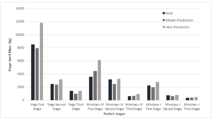
To compare the mass predicted by the performed regression with equation (4.1), the stage outer shell must be taken into account, since equation (4.1) includes the shell mass. Observing figure 4.3, the regression model provides more accurate predictions than equation (4.1) in the majority of the cases studied. As such, the regression model will be used to calculate the inert mass of the solid core stages.

To calculate the length of the liquid phase, it is calculated as the sum of the tank and thrust chamber lengths.

Trajectory Model

• Equations of Motion
• Free Flight Phase

The force of gravity applied to the vehicle is mg, where is the vehicle mass and is the local gravitational acceleration, which at all times points toward the center of the Earth. It is important to note that the comparisons are for the entire flight duration of the vehicle. The Earth rotation is taken into account by summing the required velocity at the end of the flight [94].

The contribution velocity vector is always perpendicular to the direction of the rocket and the center of mass of the Earth.

Atmospheric Model

By recognizing the costate equations (Eq. (4.36)) as homogeneous in λ, the optimization algorithm is able to find an initial value of λ such that λ=kλλ∗(kλ >0), where the superscript ”*” indicates the actual optimal value of the associated variable . The same proportionality holds between λ and λ∗ at any time, which means that initial costate values ​​can be searched in the interval −1≤λk ≤1, which reduces the search space. To deal with optimization constraints, a popular approach consists of using a penalty function method to penalize the objective function, transforming the constrained problem into an unconstrained one.

The use of the penalty function allows building a single objective function, which can be minimized by the PSO algorithm.

Drag Model

2RT indicates the molecular velocity ratio, where T is the air temperature and R = 287.058J/kgK is the air specific gas constant. The Knudsen numbers Knc and Knf represent the Knudsen limits of continuum flow and free-molecular flow, respectively, which depend solely on the vehicle geometry. The constants (A,B) are selected to establish a smooth bridging between the continuum and the free-molecular flow regime. Rocket trajectories are typically limited by the maximum dynamic pressure, i.e. when atmospheric forces are at their maximum, compromising the structural integrity of the vehicle.

The vehicle acceleration must be carefully controlled [95], usually by throttling the engines or by carefully choosing the solid grain shape [38].

Algorithm Development

• Genetic Algorithm Implementation
• Rocket Construction and Evaluation

Most of the algorithm was developed in Python, while the trajectory model was implemented using the C language to improve speed. The rocket model assembly and analysis performance are performed during the evaluation of the genetic algorithm by the slave nodes. The evaluation module can be divided into two blocks: the rocket construction block, where the mass and dimensions of the rocket are calculated, and the trajectory optimization block, where the optimal trajectory is calculated using the PSO algorithm.

First, the algorithm proceeds to calculate the mass and dimensions of the rocket using the mass model.

MDO and Models Validation

Mass Model Validation

• Solid Rocket: Vega
• Liquid Serial Staging Rocket: Proton K
• Parallel Staging Rocket: Ariane 5 ECA

The maximum deviation is shown in the inert mass of the third stage, explained by the error in the calculated length in Table 5.3. The maximum deviation is shown in the inert mass of the second stage, with an error of 3.74% explained by the underestimation of the propellant mass. Again the calculated dimensions in Table 5.5 are less than the actual length, with a maximum relative error of less than 5%.

The parameters used to estimate mass and size are shown in Table 5.7 and the calculations of mass and size are shown in Table 5.8 and Table 5.9 respectively.

ECA Booster (each) Stage 1 Stage 2

• Testing the Trajectory Model
• Genetic Algorithm Benchmark

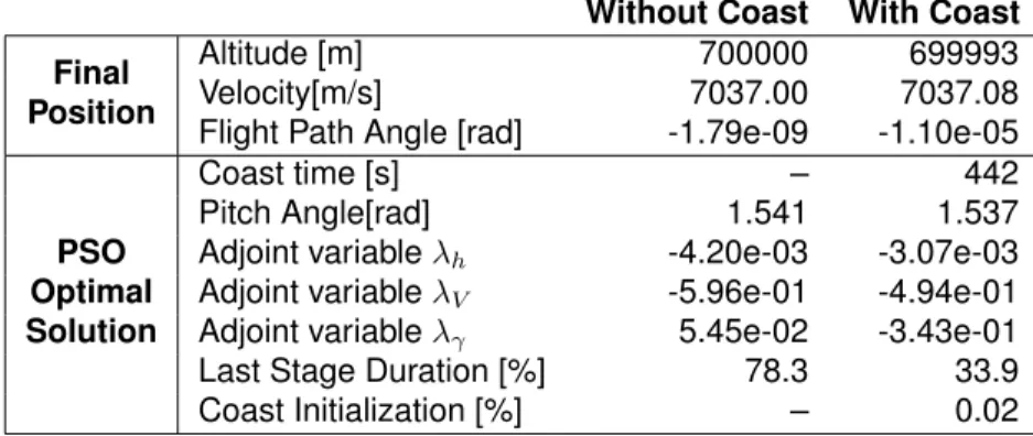
The mission and limits of the PSO optimization are shown in Tables 5.10 and 5.11, respectively. The loss due to thrust vectoring is reduced with the inclusion of the coastal phase. Both algorithms performed the optimization of the functions shown in Table 5.13 using the dimensions and space search mentioned in Table 5.14.

The results and comparison of the implemented GA and the DEAP GA are presented in Table 5.15.

Stage 2

Analyzing the imposed constraints, the TWR at liftoff has the value of 1.8 and the rocket total∆V is equal to 9092 m/s, which is within the selected range. Observing the dynamic pressure in figure 5.9, it has a maximum value of 53.5 kPa, below the imposed limit. The axial load is also below the safety load, observable in figure 5.10, using a safety factor of 1.5.

The rocket acceleration never exceeds the imposed limit of 5g0 by throttling the engine at the end of each phase, observable in figure 5.12.

Preliminary Design of a Small Launch Vehicle

Algorithm Setup

The design parameters are presented in Table 6.4, for the two- and three-stage rocket. Compared to Table 5.19, the wall thickness range set for the optimization of the small launcher is largely inferior. Thus, to prevent infeasible designs, the optimization is subject to the constraints in Table 6.5, similar to the constraints used in Section 5.3.

The parameters of both GA and PSO optimization algorithms are repeated in table 6.6 and table 6.7 respectively for convenience.

Results

The two-stage rocket has a faster increase in velocity due to performing staging later compared to the three-stage rocket, which can be visualized in Figure 6.15. The remaining speed losses due to drag and gravity are illustrated in Figure 6.10 and Figure 6.11 respectively. The axial load for the two-stage rocket and the three-stage rocket in Figure 6.14 is below the safety load, which suggests that the wall thickness can be reduced.

However, a two-stage rocket has a higher axial load applied during first thrust compared to a three-stage rocket because it has more mass and requires more thrust, as can be seen in Figure 6.15.

Stage 2 Stage 3 Two Stage

Due to the lack of information regarding the Electron's real trajectory, the trajectories are not compared. The increase in length is not only due to the fact that more space is required for the propellant mass, but also due to the smaller diameter. The larger mass value is not only due to the simplifications made in the dry mass models, but also due to the structural and propulsion assumptions (ie fixed structural material, engine number, specific impulse and propellant).

The use of a gravity turn in the trajectory model also affects the total mass of the optimal vehicle.

Conclusions

Summary and Achievements

Both designed rockets are capable of performing the mission, and the three-stage rocket offers less mass than the two-stage, as expected. The mass and size errors are due to the assumptions made, inaccuracy of the mass and size models and the use of gravitational twist in trajectory. Nevertheless, the tool is capable of performing conceptual rocket design and trajectory optimization, parallelizing the task using a master-slave architecture.

Models used by the tool can be replaced independently of other models to improve the tool in the future.

Future Developments

Behind, the trajectory optimization was tested using the Vega rocket and the reference mission in the user manual. The evolved GA was comparatively better than the DEAP GA when the feature presented more local minima and presented similar results for the remaining features. Thus, it was verified that the population with 150 individuals converged faster and obtained a rocket with a lower mass, and that all imposed restrictions were observed.

Two optimizations were carried out, involving a two-stage rocket and a three-stage rocket, to transport a payload of 150 kg to a sun-synchronous orbit at 500 km altitude.

Bibliography

Mateen, "Hammersley sampling and support-vector-regression-driven launch vehicle design," Journal of Spacecraft and Rockets, vol. Jenkins, "Design optimization of a launch vehicle for space using a genetic algorithm," Journal of Spacecraft and Rockets, vol. Betts, "Survey of numerical methods for trajectory optimization," Journal of Guidance, Control, and Dynamics, vol.

Heister, “Application of a genetic algorithm to the optimization of hybrid rockets,” Journal of Spacecraft and Rockets, vol.

Appendices

Appendix A

Regression Data