José António Silva de Carvalho Campos e Matos Uncertainty Evaluation of Reinforced Concrete and Composite Structures Behavior

To my family, especially to my grandmother Bé and to my sisters Ana Raquel and Joana, who gave me all the support;. While some introduced pattern identification techniques, others presented probabilistic estimation algorithms with updated Bayesian inference.

Introduction and motivation

This data is then used to predict structural parameters using a model identification algorithm. The same models can be used to evaluate structural performance, but now taking into account the estimated parameters.

Objectives

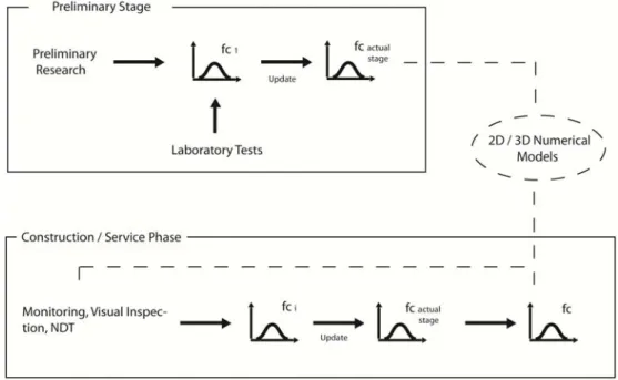
In those situations, full probabilistic estimation algorithms are recommended, as they allow introducing randomness into model parameters and evaluating structural performance from a probabilistic perspective. Therefore, within this thesis, a two-step updating algorithm has been developed, which can be successfully used to evaluate structural performance, see Figure 1.2.

Outline of thesis

Given the general problem described in expressions (2.1) to (2.3), the main concept of the SQP method is the formulation of a QP problem based on a quadratic approximation of the following Lagrangian function (2.4). In this situation, and taking into account expression (3.4), the rear is only one constant times the probability (3.6).

Optimization Algorithms

Optimization algorithms

In a more advanced formulation, the objective function f(x) to be minimized or maximized may be subject to constraints. An efficient and accurate solution to this problem depends not only on the size of the problem in terms of the number of constraints and design variables, but also on the characteristics of the objective function and constraints.

Local optimization methods

Sequential quadratic programming

Updating the Hessian matrix
Quadratic programming solution
Line search and objective function

Each iteration (2.8) calculates a positive final quasi-Newton approximation of the Hessian of the Lagrangian function (2.4). The feasible subspace for dk is formed from a basis Zk whose columns are perpendicular to the estimate of the active set Āk.

Global optimization methods

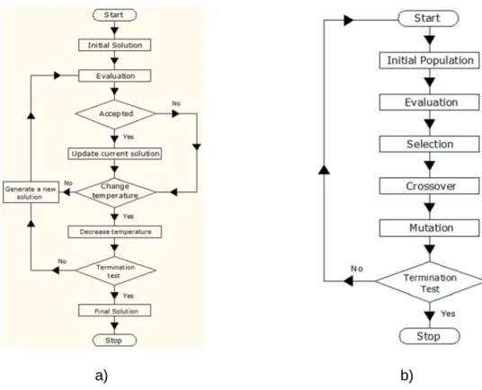
Simulated annealing
Genetic algorithm
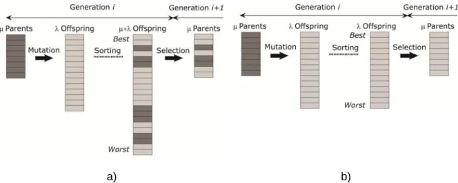
Evolutionary strategies

Initial parent population
Recombinant operator
Mutation operator
Selection operator
Tolerance criteria

At each iteration, a new random point is generated around the current point according to the neighborhood function. Evolutionary Strategies (ES) is a global search algorithm based on Darwinian natural evolution and the concept of survival of the fittest.

Example

Function 3

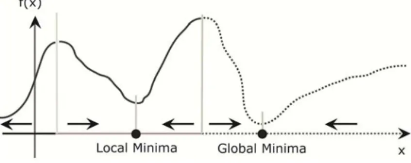
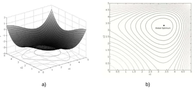
The second test function is a composite 2D polar coordinate function with several local minima and a clear global minimum. From the first analysis, it can be stated that all global search algorithms give very good results.

Real application

Experimental test
Numerical model
Obtained results

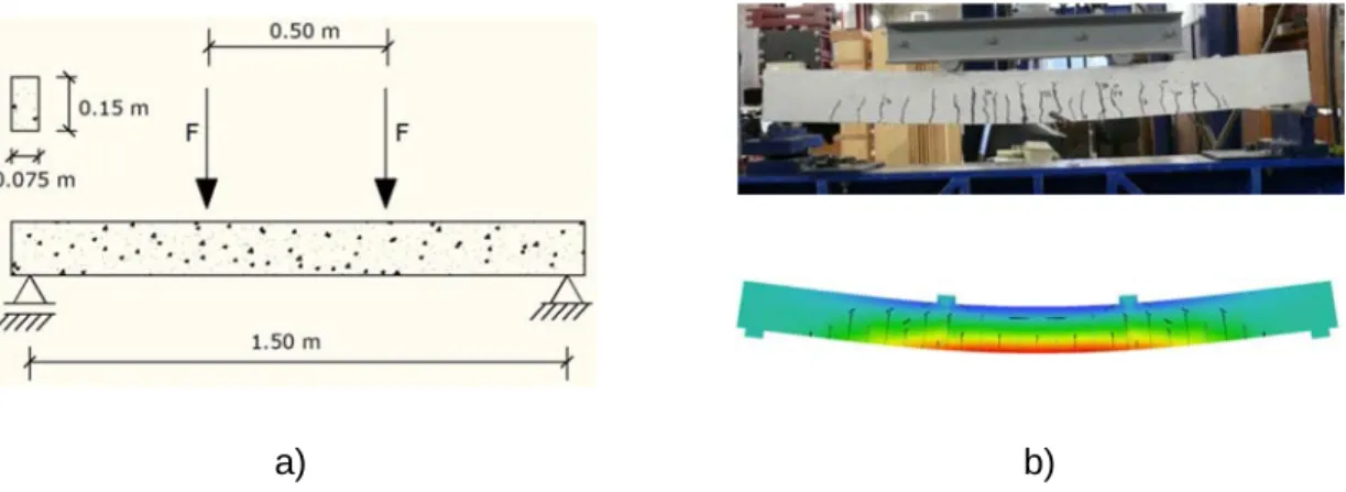
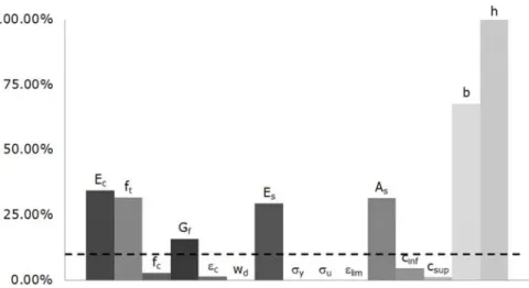
In Figure 2.12, the applied load is plotted against the midspan displacement for experimental and numerical results, considering each optimization algorithm. (5) section dimensions are generally less than nominal values; (6) inferior concrete cover values (cinf) are close to each other and to the nominal.

Conclusions

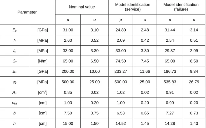
From the first analysis of table 5.6. it can be found that: (1) The obtained value of some parameters such as tensile (ft) and compressive strength of concrete (fc), section width (b). The uncertainty of the measured reaction component of the fitness function must then be determined. Applying Bayesian inference to the obtained values from model identification in the service phase yields the results given in Figure 5.24.

Bayesian Inference

Bayes theorem

As more data is collected, Bayesian analysis is used to update the prior distribution into a posterior distribution. In this situation, the prior and the posterior distributions of Θ are respectively represented by density functions, p(Θ) and p(Θ|x). Consequently, Bayes' theorem consists in multiplying the prior and the probability and then normalizing them to get the posterior distribution.

Prior distributions

This is the negative expectation of the second derivative of the log-likelihood, LogL(Θ), and measures the curvature of the likelihood function. This prior is not dominated by the likelihood and has an impact on the posterior distribution. The property that the posterior distribution follows the same parametric form as the prior distribution is called conjugation.

Bayesian inference

Normal data with unknown mean (µ) and known variance (σ 2 ): Jeffrey’s prior….… 41
Normal data with unknown mean (µ) and variance (σ 2 ): conjugate prior

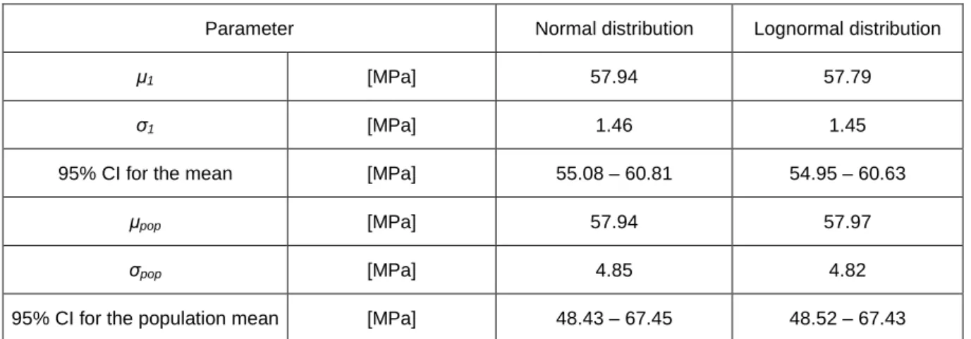
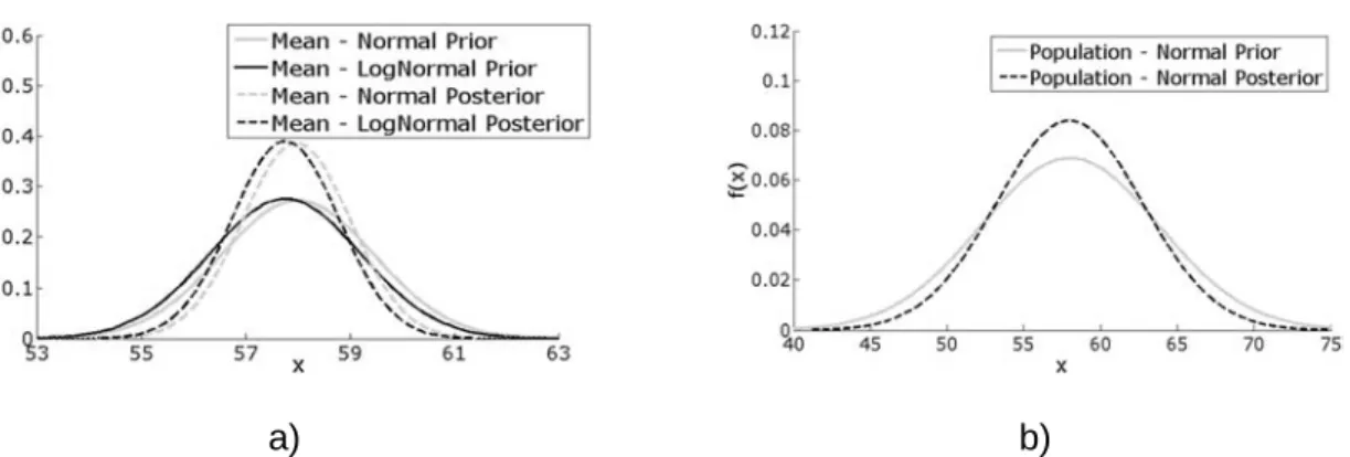
The posterior distribution of the mean, given data x, is thus a normal with mean x (µ1) and variance σ2/n (σ12). The posterior population mean is equal to µ1 (µpop), while its variance (σpop2) is obtained through (3.27). The posterior population mean is equal to µ1 (µpop), while its variance (σpop2) is obtained through (3.40).

Posterior simulation

The parameters of the posterior distribution thus combine the prior information with that contained in the new data. Accordingly, in this situation, the sampler starts with an initial value of ν0 and S0 and obtains 1/σ2 from the marginal posterior distribution (3.43). The sampler then uses the value of 1/σ2 to generate a new value of µ calculated from the conditional posterior distribution of the mean with respect to the variance (3.44).

An application of Bayesian inference framework

Statistical analysis of data
Normal data with unknown mean (µ) and known variance (σ 2 )
Normal data with unknown mean (µ) and variance (σ 2 )

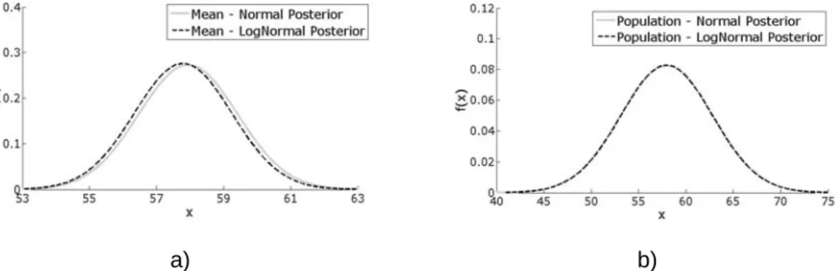
The results obtained for the posterior distribution of the mean are closer together for both the normal and log-normal distributions. In addition, it can be observed that the log-normal distribution has a slightly lower mean value than the normal distribution for both earlier and later distributions. The results obtained for the posterior distribution of the mean are identical for both normal and log-normal cases.

Alternative updating methodology using Weibull distribution…

The Weibull distribution
The proposed methodology
Obtained results

One of the most suitable methods is to perform the curve fitting to the histogram of data. The standard deviation value was considered to be related to the 95% confidence interval of the Weibull analysis regression parameters. Therefore, it is calculated as the distance between the mean and the upper or lower bound of the confidence interval.

Uncertainty sources

From the analysis, it is possible to conclude that the results from model identification up to and including failure load are those that best fit the experimental curve. From the analysis, it is possible to conclude that the results from model identification up to and including failure load are those that best fit the experimental curve. It is possible to identify that the obtained resistance PDF with values from model identification to failure load is located between the others.

The obtained resistance PDF with the values from the model identification in the service phase gives the highest mean. For each analysis, a model is obtained, respectively taking into account the nominal values and those from the identification of the model at the service stage and up to the failure load.

Structural assessment levels

Probabilistic assessment

The main result of this method is an updated resistance PDF of the evaluated structure. The main purpose of model identification is to obtain the most likely values of model parameters. To calculate the numerical model, the non-linear structural analysis software ATENA® [24] is used.

Sensitivity analysis

The following procedure is therefore recommended: (1) develop the deterministic numerical model of analyzed structure using mean values of input parameters; (2) to divide the structural parameters by category (material, geometric, physical) and subcategory (concrete, steel, interface, support, …); (3) for each parameter, to determine the most suitable CV; (4) varying each parameter by adding or subtracting a standard deviation value, keeping all other parameters fixed; (5) for each set of parameter values to proceed to the numerical analysis with a nonlinear structural analysis software; (6) to use the following expression.

Model identification

Optimization algorithm
Errors

Measurement
Modelling

Convergence criterion
Engineering judgment procedure

According to Figure 4.3, an established stopping criterion for model identification algorithm is the convergence criterion for the fitness function, given by expression (4.4). There are several options for applying the fitness function convergence criterion for model identification (Figure 4.3). In this situation, the convergence criterion defines that the improvement in the fitness function value (∆f) from two models separated by a predetermined gap (n) must be lower than or equal to a threshold value (ε), indicated by Figure 4.3.

Probabilistic analysis

Randomness

Material
Geometry
Physic

Bayesian inference
Simulation algorithms

It defines the number of samples generated, each PDF type parameter and the correlation matrix. This method limits the total number of samples, N, to the number of intervals taken into account in the sampling area distribution, k. The advantage of this method is that the number of simulations can be reduced while maintaining the same numerical precision.

Structural performance indexes

Evaluation assessment
Safety assessment

The assessment of structural safety consists of calculating the obtained reliability index and comparing it with a target reliability index (βtarget). Target reliability values should be determined based on the reliability analysis of many structures. The AASHTO LRFR code [2] proposes a target reliability index value for strength assessment of bridge members, βtarget = 2.50.

Conclusions

The average value, the nominal values and those from the model identification in the service phase and up to the failure load were taken into account. The average PDF values were the nominal values and those from the model identification in the service phase and up to the failure load. The reduction of the β-value is verified by taking into account the value from the model identification in the service phase.

Reinforced Concrete Beams

Pinned-fixed beams

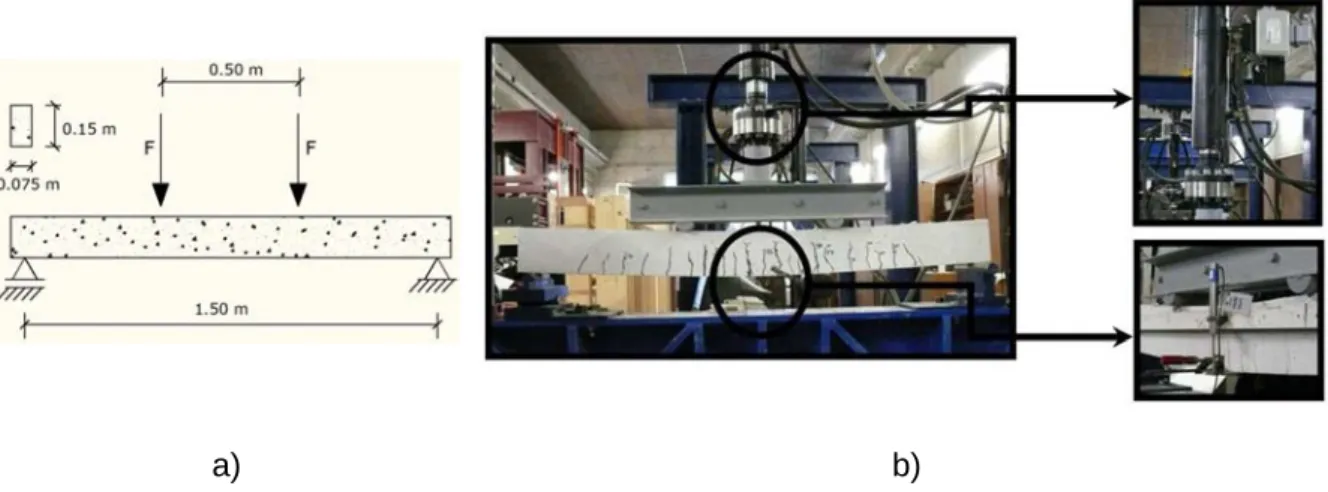
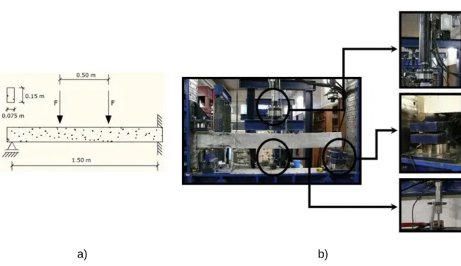
The pinned support reaction was registered by a load cell with 200 kN capacity and 0.10% accuracy. Due to the fact that it is one degree hyperstatic, the collapse mechanism is characterized by. As the applied load and the pinned support reaction were measured, it was possible to indirectly obtain the bending moment at fixed support using the static equilibrium equations. a) b).

Numerical analysis

Pinned-pinned beams
Pinned-fixed beams

Two different load cases were adopted respectively, one representing the actual supports and other the applied displacement. The midspan displacement, the applied load and the pinned support reaction were monitored during the analysis. The reference model is the same as the one used to determine the applied load error.

Model identification

A first analysis allows to conclude that the value of the fitness function obtained in the service phase is lower than that determined until failure loading. It is verified that the fitness function value obtained in the service phase is lower than that determined until failure loading. The achieved error from model identification to the error load is lower than that given by nominal values and by model identification in the service phase.

Characterization tests

Concrete material
Steel material
Concrete cover

In fact, it can be verified that when using the methodology in the service phase, the model identification is performed for this region, where the curve fit for the failure region cannot be guaranteed. The error obtained for the model identification situation as long as the error loading is less than 10%, which is reasonable. Also shown is the bias value, which represents the ratio between the experimental and the nominal value.

Probabilistic analysis

(3) The p-index obtained with nominal values is closer to that obtained with values from model identification in the service phase. The obtained resistance PDF with nominal values is close to that obtained with values from model identification to failure load. When applying Bayesian inference to the values obtained from model identification to failure load, the results given in Figure 5.26 are obtained.

Safety assessment

An increase in the β value is verified when considering the values of model identification in service phase. Accordingly, the most accurate result is the one that takes into account the values from model identification to failure load. In this case, the load intensity (FR1), required to obtain MR1*, is calculated via equation (5.31).

Conclusions

By analyzing this table, it is possible to conclude that obtained β value considering the values from model identification to failure load is lower than the one considering nominal values. Some conclusions were obtained from probabilistic assessment: (1) model identification until failure load gives very good results (errors less than 10%); (2) model identification in service phase only gives good results for service region. Complementary tests are therefore recommended in this situation; (3) the most accurate models from a probabilistic analysis are those with values from model identification to failure load.