ENTROPY SPECTRUM OF LYAPUNOV EXPONENTS
L. J. D´IAZ, K. GELFERT, AND M. RAMS
Abstract. We study the fiber Lyapunov exponents of step skew-product maps over a complete shift ofN, N ≥ 2, symbols and withC1 diffeomor- phisms of the circle as fiber maps. The systems we study are transitive and genuinely nonhyperbolic, exhibiting simultaneously ergodic measures with pos- itive, negative, and zero exponents. We derive a multifractal analysis for the topological entropy of the level sets of Lyapunov exponent. The results are formulated in terms of Legendre-Fenchel transforms of restricted variational pressures, considering hyperbolic ergodic measures only, as well as in terms of restricted variational principles of entropies of ergodic measures with given exponent. We show that the entropy of the level sets is a continuous function of the Lyapunov exponent. The level set of zero exponent has positive, but not maximal, topological entropy. Under the additional assumption of proxi- mality, there exist two unique ergodic measures of maximal entropy, one with negative and one with positive fiber Lyapunov exponent.
Contents
1. Introduction 2
2. Statement of the results 4
3. Setting 9
3.1. Axioms 9
3.2. Previous results from [DGR2] 10
4. Entropy, pressures, and variational principles 11
4.1. Entropy: restricted variational principles 12
4.2. Pressure functions 13
4.3. The convex conjugate of the pressure function 15
5. Exhausting families 16
6. Homoclinic relations and construction of exhausting families 18
6.1. Homoclinic relations 18
6.2. Existence of exhausting families 19
7. Proof of Theorem 1. Entropy spectrum 20
7.1. Measure(s) of maximal entropy 21
7.2. The level sets with negative/positive exponents 21
2000Mathematics Subject Classification. 37D25, 37D35, 37D30, 28D20, 28D99.
Key words and phrases. entropy, ergodic measures, Legendre-Fenchel transform, Lyapunov exponents, pressure, restricted variational principles, skew-product, transitivity.
This research has been supported [in part] by CNE-Faperj, CNPq-grants (Brazil), and EU Marie-Curie IRSES “Brazilian-European partnership in Dynamical Systems” (FP7-PEOPLE- 2012-IRSES 318999 BREUDS). The authors acknowledge the hospitality of IMPAN, IM- UFRJ, and PUC-Rio. MR was partially suported by National Science Centre grant 2014/13/B/ST1/01033 (Poland).
1
arXiv:1610.07167v1 [math.DS] 23 Oct 2016
7.3. The level sets with zero and extremal exponents 22 8. Proof of Theorem 2. Measures of maximal entropy 28
8.1. Synchronization 28
8.2. End of the proof of Theorem 2 29
8.3. Proof of Corollary 3 29
9. Proof of Theorem 5. Shapes of pressure and Lyapunov spectrum 30
Appendix. Entropy 31
References 31
1. Introduction
We will study the entropy spectrum of Lyapunov exponents, that is, the topolog- ical entropy of level sets of points with a common given Lyapunov exponent. This subject forms part of the multifractal analysis which, in general, studies thermody- namical quantities and objects (such as, for example, equilibrium states, entropies, Lyapunov exponents, Birkhoff averages, and recurrence rates) and their relations with geometrical properties (for example, fractal dimensions). Those properties are often encoded by the topological pressure.
In the uniformly hyperbolic context multifractal analysis is understood in great depth and has found already far reaching applications. There is a huge litera- ture on this subject. To highlight a collection of results in the field at different stages of development, we refer, for example, to [R] (analyticity of pressure and its consequences), [O, PW] (multifractal analysis for conformal expanding maps and Smale’s horsehoes), and [BS] (mixed spectra and restricted variational principles).
In many of those references, particular attention is drawn to so-called geometric potentials because of their close relation to Lyapunov exponents, entropy, and SRB measures. Two key properties of uniformly hyperbolic systems, under which the classical context of multifractal analysis was developed so far, are the specification property (studied for example in [TV, PS, FLP]) and the existence and uniqueness of equilibrium states.
The multifractal analysis theory extends also to “one-sided” nonuniformly hy- perbolic systems, that is, for example to nonuniformly expanding maps where the presence of a nonpositive Lyapunov exponent is the only obstruction to hyperbol- icity, that is, the spectrum of Lyapunov exponents covers a range of hyperbolicity and the zero exponent bounds this range from one side, see for example [GPR] (ex- pansive Markov maps of the interval) and [PR, IT] (multimodal interval maps). So far, there is not much understanding of a multifractal analysis for more complicated types of nonhyperbolic systems. It is difficult to describe all the situations that can happen in general; one natural class of systems to focus on could be the systems with a designated line field (associated with the Oseledets decomposition) for which the Lyapunov exponent takes both positive and negative values arbitrarily close to zero. Naturally, we assume topological transitivity, hence the system in question cannot split into “one-sided” nonuniformly hyperbolic parts.
Probably, the simplest setting of such a “two-sided” nonhyperbolic dynamical system is a step skew-product with a hyperbolic horseshoe map in its base and circle diffeomorphisms in its fibres. The nonuniform hyperbolicity arises from the coex- istence of contracting and expanding regions which are blended by the dynamics.
The system exhibits ergodic measures which positive and negative fiber Lyapunov exponents. An important feature is the occurrence of ergodicnonhyperbolic mea- sures (i.e., with zero Lyapunov exponent) with positive entropy. The considered dynamics is topologically transitive and simultaneously has “horseshoes” which are contracting and “horseshoes” which are expanding in the fiber direction. More- over, these horseshoes are intermingled and there coexist dense sets of periodic points with negative and positive fiber Lyapunov exponents. The precise setting is discussed in Section 3.
The present paper is a continuation of [DGR2] where properties of the space of invariant measures were investigated. Here we will concentrate on the multi- fractal analysis of the entropy of the level sets of fiber Lyapunov exponents. We follow a thermodynamic approach based on a restricted variational principle. The philosophy is that to obtain relevant multifractal information about the respective class of exponents one should not consider the whole variational-topological pres- sure, but instead its restrictions to ergodic measures with corresponding exponents, so-calledrestricted pressures. The use of restricted (sometimes also calledhidden) pressures was initiated in [MS] (for rational maps of the Riemann sphere) and subsequently used, for example, in [GPR] (for non-exceptional rational maps) and [PR] (for multimodal interval maps). As the difficulty in our setting comes from the coexistence of negative, zero, and positive fiber Lyapunov exponents and as zero exponent measure are notoriously difficult to analyze, a natural solution is to consider the restricted pressures defined on the ergodic measures with negative and positive exponents, respectively (it turns out that zero exponent ergodic measures do not play a significant role). This approach is made possible by the fact that the uniformly hyperbolic subsystems with negative/positive Lyapunov exponents (but not the system as the whole) satisfy the specification property.
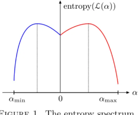
Summarizing our results: the spectrum of Lyapunov exponents is a closed inter- val [αmin, αmax] that contains zero in its interior. For eachα∈[αmin, αmax] the level set L(α) of points with fiber exponent equal toαis nonempty and its topological entropy changes continuously withα(see Figure 1). The entropy spectrum of fiber
entropy(L(α))
0 α
αmin αmax
Figure 1. The entropy spectrum
Lyapunov exponents is described in terms of those restricted pressure functions and their respective Legendre-Fenchel transforms.
To obtain our results, we combine a thermodynamical and an orbitwise approach.
On the one hand, we study the restricted variational pressure functions and extract properties from its shape. Here, one of the big selling points of this approach is that it gives us convexity for free, which turns out to be a surprisingly useful
property. On the one hand, in our approach we put our hands on the orbits of the level sets (the amount of their entropy provides explicit information about them), using natural recurrence properties of the systems (which is guided by the concept of so-called blending intervals in [DGR2]), and follow the “orbit-gluing approach”
(which lead us to the notion of skeletons of the dynamics in [DGR2]). We point out that we always work in the lowest possible regularity and consider C1 circle diffeomorphisms as fiber maps.
Let us return to the discussion of the zero Lyapunov exponent. The greatest obstacle in our investigation, as usual in the study of nonhyperbolic systems, are points and measures with zero exponent. While for nonzero exponents we can give the full description of the Lyapunov exponent level sets, including the restricted variational principle and the exact formula for their entropy, we have very restricted tools for studying the zero exponent level set L(0). We are able to describe the entropy of this set, but the restricted variational principle cannot be obtained by our methods. Let us observe that the fact that L(0) has positive topological entropy was obtained in a similar context in [BBD] by proving the existence of ergodic measures with positive entropy and zero exponents. In this paper this property is obtained as a surprising consequence of the shape of the pressure map. Though positive, we also show that the topological entropy ofL(0) is strictly smaller than the maximal, that is, the topological entropy of the system.
The systems we study always have (at least) two hyperbolic ergodic measure of maximal entropy, one with negative and one with positive fiber Lyapunov expo- nent. Indeed, this is an immediate consequence of [C], obtained from a different point of view of our system as a random dynamical system, that is, as a product of independent and identically distributed circle diffeomorphisms, also observing the fundamental fact that our hypotheses exclude the case that our system is a rotation extension of a Bernoulli shift. It is a particular case of a result in a more general setting [RH2TU], stated for accessible partially hyperbolic diffeomorphisms having compact center leaves, see also [TY]. Under the additional assumption of proxi- mality, with [Ml] we even can conclude uniqueness of ergodic measure of maximal entropy with negative and positive exponents.
Finally, we point out that the systems that we study are models for robustly tran- sitive and nonhyperbolic diffeomorphisms and sets with compact central leaves [BDU, RH2TU]. From another point of view, which in fact provides some of our tools, the systems can be also considered as actions of a group of diffeomorphisms on the circle or as random dynamical systems.
2. Statement of the results
Letσ: ΣN →ΣN,N≥2, be the usual shift map on the space ΣN ={0, . . . , N− 1}Zof two-sided sequences. We equip the shift space ΣN with the standard metric d1(ξ, η) = 2−n(ξ,η), where n(ξ, η) = sup{|`|: ξi =ηi fori =−`, . . . , `}. We equip ΣN ×S1 with the metric d((ξ, x),(η, y)) = sup{d1(ξ, η),|x−y|}, where |·| is the usual metric onS1.
Consider a finite family fi: S1 → S1, i = 0, . . . , N−1, of C1 diffeomorphisms and the associated step skew-product
(2.1) F: ΣN ×S1→ΣN ×S1, F(ξ, x) = (σ(ξ), fξ0(x)).
We will consider a class of maps which are topologically transitive and “nonhy- perbolic in a nontrivial sense that there are some “expanding region” and some
“contracting region” (relative to the fiber direction) and that any of those can be reached from anywhere in the ambient space under forward/backward iterations.
More precisely, we will requireFto satisfy Axioms CEC±and Acc±(see Section 3).
LetMbe the space ofF-invariant probability measures supported in ΣN ×S1, equip Mwith the weak∗ topology, and denote byMerg⊂Mthe subset of ergodic measures. To characterize nonhyperbolicity, givenµ∈Mdenote byχ(µ) its(fiber) Lyapunov exponent which is given by
χ(µ)def= Z
log|(fξ0)0(x)|dµ(ξ, x).
An ergodic measure µ is nonhyperbolic if χ(µ) = 0. Otherwise the measure is hyperbolic. In our setting any hyperbolic ergodic measure has either a negative or a positive exponent. Accordingly, we split the set of all ergodic measures and consider the decomposition
(2.2) Merg=Merg,<0∪Merg,0∪Merg,>0
into measures with negative, zero, and positive fiber Lyapunov exponent, respec- tively. In our setting, each component is nonempty. In general, it is very diffi- cult to determine which type of hyperbolicity “prevails”. For that we will study the spectrum of possible exponents and will perform a multifractal analysis of the topological entropy of level sets of equal (fiber) Lyapunov exponent.
To be more precise, a sequence ξ = (. . . ξ−1.ξ0ξ1. . .) ∈ ΣN can be written as ξ=ξ−.ξ+, whereξ+∈Σ+N def={0, . . . , N−1}N0 andξ− ∈Σ−N def={0, . . . , N−1}−N. Givenfinite sequences (ξ0. . . ξn) and (ξ−m. . . ξ−1), we let
f[ξ0... ξn] def=fξn◦ · · · ◦fξ0 and f[ξ−m... ξ−1.] def= (f[ξ−m... ξ−1])−1. Forn≥0 denote also
fξndef=f[ξ0... ξn−1] and fξ−ndef=f[ξ−n... ξ−1.].
GivenX = (ξ, x)∈ΣN ×S1consider the(fiber) Lyapunov exponent ofX χ(X)def= lim
n→±∞
1
nlog|(fξn)0(x)|,
where we assume that both limitsn → ±∞exist and coincide. Note that in our context the exponent is nothing but the Birkhoff average of the continuous function (also calledpotential)ϕ: ΣN×S1→Rdefined for X= (ξ, x) by
(2.3) ϕ(X)def= log|(fξ0)0(x)|.
We will analyze the topological entropy of the following level sets of Lyapunov exponents: givenα∈Rlet
L(α)def=
X ∈ΣN×S1:χ(X) =α
assuming that the Lyapunov exponent atX is well defined and equal to α. Note that each level set is invariant but, in general, noncompact. Hence we will rely on the general concept of topological entropyhtop introduced by Bowen [B1] (see Appendix). Denoting byLirr the set of points where the fiber Lyapunov exponent
is not well-defined (either one of the limits does not exist or both limits exist but they do not coincide), we obtain the followingmultifractal decompositionof ΣN×S1
ΣN×S1= [
α∈R
L(α)∪Lirr.
Note thatL(α) will be nonempty in some range ofα, only. Under our axioms this range decomposes into three natural nonempty parts
{α:L(α)6=∅}= [αmin,0)∪ {0} ∪(0, αmax], where
αmax
def= max
α: L(α)6=∅ , αmin
def= min
α:L(α)6=∅ . It is easy to verify that max and min are indeed attained.
To state our main results, we need the following thermodynamical quantities.
Denote by h(µ) the entropy of a measure µand consider the pressures and their convex conjugates (see Section 4 for details)
(2.4) P∗(qϕ)def= sup
µ∈Merg,∗
h(µ)−qχ(µ)
, E∗(α)def= inf
q∈R
P∗(qϕ)−qα , where ∗ should be replaced by < 0 and > 0, respectively. In the terminology of [PRS], this would be called (positive/negative)variational hyperbolic pressure, we call it simplypressure. For simplicity we will use the notation
P∗(q)def=P∗(qϕ),
as this is the only family of potentials whose pressure we are going to consider.
Similarly, we define
P0(q)def= sup
µ∈Merg,0
h(µ).
Clearly,
max{P<0(q),P0(q),P>0(q)}=Ptop(qϕ)
is the classicaltopological pressure ofqϕ with respect toF (see [Wa, Chapter 7]).
We will also write E for both E>0 and E<0, because the domains of those two functions are disjoint.
Theorem 1. Consider a transitive step skew-product mapF as in (2.1)whose fiber maps areC1. Assume that F satisfies Axioms CEC±and Acc±.
Then for everyα∈[αmin, αmax] we haveL(α)6=∅. Moreover,
• for everyα∈(αmin,0) we have htop(L(α)) = sup
h(µ) :µ∈Merg, χ(µ) =α =E<0(α),
• for everyα∈(0, αmax)we have htop(L(α)) = sup
h(µ) :µ∈Merg, χ(µ) =α =E>0(α),
• for everyα∈ {αmin,0, αmax} we have
β→αlim htop(L(β)) =htop(L(α)),
• htop(L(0))>0.
Moreover, there exist (finitely many) ergodic measuresµ+, µ− of maximal entropy h(µ±) = logN and with χ(µ−)<0< χ(µ+).
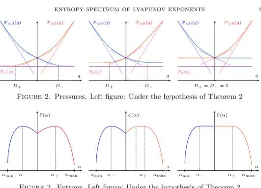
D+ D−
P>0(q)
P<0(q)
P0(q)
q
D+ D−
P>0(q)
P<0(q)
P0(q)
q
D+=D−= 0
P>0(q)
P<0(q)
P0(q)
q
Figure 2. Pressures. Left figure: Under the hypothesis of Theorem 2
E(α)
α
α− α+
αmin αmax
E(α)
α
α− α+
αmin αmax
E(α)
α
α− α+
αmin αmax
Figure 3. Entropy. Left figure: Under the hypothesis of Theorem 2 To prove uniqueness of the measures µ± of maximal entropy, we require an additional assumption (see Section 8.1 for discussion). We say that the IFS is proximal if for everyx, y∈S1 there exists at least one sequenceξ∈ΣN such that
|fξn(x)−fξn(y)| →0 as|n| → ∞.
It is easy to see that the IFS is proximal if, for example, it contains a map with one attracting and one contracting fixed point (contraction-expansion map; North pole-South pole map) and the IFS satisfies our other axioms CEC±and Acc±.
Theorem 2. Assume the hypothesis of Theorem 1. Assume also that the IFS is proximal. Then there exist unique ergodicF-invariant probability measuresµ− and µ+ of maximal entropy h(µ±) = logN, respectively, and satisfying
α−def=χ(µ−)<0< α+
def=χ(µ+).
We have
htop(L(α−)) =htop(L(α+)) = logN and
htop(L(α))<logN for allα6=α−, α+.
Similar phenomenon as in Theorem 2 (the entropy achieving its maximum away from zero exponent) in a slightly different setting (for ergodic measures on C2 systems) was observed in [TY]. The weak∗ and entropy convergence means that the sequence of measures converges in the weak∗topology and their entropies also converge to the entropy of the limit measure.
Corollary 3. Under the hypothesis of Theorem 2 no measure which is a nontrivial convex combination of the two ergodic measures of maximal entropy is a weak∗and in entropy limit of ergodic measures.
The results in [TY] and our results suggests the following conjecture (which is indeed true for maximal entropy measures, by Corollary 3).
Conjecture 4. For every pair of hyperbolic ergodic measures µ1 and µ2 with χ(µ1) < 0 < χ(µ2) every nontrivial convex combination of µ1 and µ2 cannot be approximated (weak∗ and in entropy) by ergodic measures.
Under the hypothesis of Theorem 2, the graph of the Lyapunov spectrum α→ htop(L(α)) =E(α) is as on Figure 3 (left figure). Under the hypothesis of Theo- rem 1, possible shapes of the graph of the corresponding Lyapunov spectrum are as on Figure 3 (middle and right figures).
We summarise the properties of (restricted) pressure functions, its Legendre- Fenchel transform, and of the Lyapunov spectrum in the following theorem (com- pare Figures 2 and 3).
Theorem 5. Under the assumptions of Theorem 1,
a) P<0andP>0 are nonincreasing and nondecreasing convex functions, respec- tively,
b) (Plateaus) There are numbersD± andh± such that
P<0(q) =h− for allq≥D− and P>0(q) =h+ for allq≤D+. c) h−=h+=htop(L(0)),
d) D+≤0≤D−,
e) P>0(0) =P<0(0) = logN =htop(F),
f) α7→htop(L(α))achieves its maximum valuelogN at some points α−<0 and α+>0,
g) Forα <0 the functionα7→ E(α) is a Legendre-Fenchel transform of q 7→
P<0(q). Similarly, for α >0 the function α7→E(α) is a Legendre-Fenchel transform ofq7→P>0(q). In particular,α7→E(α)is a concave function on the domainsα <0 andα >0, respectively,
h) htop(L(α))is a continuous function on[αmin, αmax], i) 0≤DRE(0)<∞and 0≤ −DLE(0)<∞,
j) htop(L(0))>0.
Moreover, under the assumptions of Theorem 2 we have additional properties k) P>0(q) andP<0(q)are differentiable atq= 0,
in items d) and i) we have strict inequalities:
D+<0< D− and DLE(0)<0< DRE(0),
and the pointsα−, α+ in item f ) are the unique numbersαfor whichhtop(L(α)) = logN.
Remark 2.1. The following questions remain open. The restricted pressures can be differentiable or nondifferentiable at the beginning of the plateaus in Theorem 5 item b). The nondifferentiability of, for example, P>0 at a− would mean that E(α) is linear on some interval [0, q]. Further regularity properties (smoothness, analyticity) of the restricted pressure functions (excluding the ends of plateaus) and of the spectrum are unknown.
The asymptote ofP>0atq→ ∞is some line{P =αmaxq+hmax}, similarlyP<0
is asymptotic to{P =αminq+hmin}, and we do not know whetherhmax andhmin
are equal to zero (which would mean thathtop(L(αmax)) =htop(L(αmin)) = 0; this phenomenon is sometimes referred to asergodic optimization, see for example [J]).
Finally, we do not know if there exist ergodic measures with Lyapunov expo- nent zero and with entropy arbitrarily close tohtop(L(0)) (Variational principle for exponent zero).
Our approach is to treat positive, negative, and zero spectra separately. First, we recall the restricted variational principle for entropy which provides a lower bound forhtop(L(α)), see Section 4.1. Then we show that these values can be expressed via the Legendre-Fenchel transform of the restricted pressure function in (2.4) (treating negative and positive values separately). For that we will strongly use that for any pair of uniformly hyperbolic sets with negative (positive) fiber exponents we can find a larger one containing them both and hence we can gradually approximate from below the restricted pressure P<0 (P>0), see Section 5. Finally, using the existence of so-called skeletons established in [DGR2], for any αwith a level set of given entropy hwe can construct hyperbolic sets with entropy close to hwith almost homogeneous exponents close toα. This will show thathtop(L(α)) is limited from above by entropies of ergodic measures with exponents close toα. Concavity of the Legendre-Fenchel transform implies its continuity, which concludes the main argument.
The structure of this paper is as follows. In Section 3 we recall the most impor- tant properties of the systems we investigate, obtained in [DGR2]. In Section 4 we give some basic information about the thermodynamical formalism. In Section 5 we introduce (in an abstract setting) the restricted pressures and exhausting families, then in Section 6 we construct them in the setting of our paper. Finally, in the last three sections we prove our three theorems.
3. Setting
We recall the precise setting of our axioms CEC± and Acc± and their main consequences, established in [DGR2]. The step skew-product structure ofF allows us to reduce the study of its dynamics to the study of the iterated function system (IFS) generated by the fiber maps{fi}Ni=0−1. In what follows we always assume that F is transitive.
3.1. Axioms. Given a pointx∈S1, consider and define itsforward andbackward orbits by
O+(x)def= [
n≥0
[
(θ0...θn−1)
f[θ0... θn−1](x) andO−(x)def= [
m≤1
[
(θ−m...θ−1)
f[θ−m... θ−1.](x), respectively. Consider also thefull orbit ofx
O(x)def=O+(x)∪ O−(x).
Similarly, we define the orbitsO+(J),O−(J), andO(J) for any subsetJ⊂S1. In requiring that the underlying IFS {fi} of the map F satisfies the axioms CEC±and Acc±we mean that there are so-called (closed)forward and backward blending intervals J+, J−⊂S1 such that the following properties hold.
CEC+(J+) (Controlled Expanding forward Covering relative to J+).
There exist positive constants K1, . . . , K5 such that for every interval H ⊂ S1 intersectingJ+ and satisfying|H|< K1 we have
• (controlled covering) there exists a finite sequence (η0. . . η`−1) for some pos- itive integer`≤K2|log|H||+K3 such that
f[η0... η`−1](H)⊃B(J+, K4), whereB(J+, δ) is theδ-neighbourhood of the setJ+.
• (controlled expansion) for everyx∈H we have log|(f[η0... η`−1])0(x)| ≥`K5.
CEC−(J−) (Controlled Expanding backward Covering relative to J−).
The IFS{fi−1}satisfies the Axiom CEC+(J+).
Acc+(J+) (forward Accessibility relative to J+). O+(intJ+) =S1. Acc−(J−) (backward Accessibility relative to J−). O−(intJ−) =S1.
When the step skew-product F is transitive then there is a common interval J ⊂S1 satisfying CEC±(J) and Acc±(J) (see Lemma 3.5 and detailed discussion in [DGR2, Section 2.2]).
In what follows we recall some properties of the IFS{fi}and the skew-product mapF satisfying the axioms above that will be used in this paper.
3.2. Previous results from[DGR2]. A technical result that we extract from [DGR2] claims that given an ergodic measure µwith exponentχ(µ) =α >0 and entropy h(µ) >0, for every small β <0 there are ergodic measures with exponents close to β and positive entropy, but in this construction some entropy is lost. [DGR2, Theorem 5] bounds the amount of lost entropy that is related to the size ofα+|β|.
A specially interesting case occurs when the exponent β is taken arbitrarily close to 0−. The estimates in [DGR2, Theorem 5] are summarized in the next lemma.
Lemma 3.1 (Rephrasing partially [DGR2, Theorem 5]). There exists c >0 such that for every ergodic measure µ with nonzero Lyapunov exponent χ(µ) = α6= 0 there is a sequence of ergodic measures νi with Lyapunov exponents χ(νi) = βi, sgnα6= sgnβi, such that βi→0 and
i→∞lim h(νi)≥ h(µ) 1 +c|α|. This result also implies the following.
Corollary 3.2. There exist ergodic measures with exponents arbitrarily close to0+ and0−.
The systems considered in this paper satisfy the so-calledskeleton propertywhich implies the existence of orbit pieces that allow to approximate entropy and Lya- punov exponent, see [DGR2, Section 4] for details. The skeleton property is referred to some blending interval and to quantifiers corresponding to the entropy and a level set for the Lyapunov exponent. An important property is that ifL(α)6= 0 then the skeleton property holds relative to h=htop(L(α)) and α. Based on the skeleton property, we have the following.
Given a compactF-invariant set Γ⊂ΣN ×S1, we say that Γ hasuniform fiber expansion (contraction) if every ergodic measureµ∈M(Γ) has positive (negative) Lyapunov exponent. It is hyperbolic if it either has uniform fiber expansion or
uniform fiber contraction. We say that a set is basic (with respect toF) if it is compact,F-invariant, locally maximal, topologically transitive, and hyperbolic1. Proposition 3.3 ([DGR2, Theorems 4.3 and 4.4]). Givenα6= 0such thatL(α)6=
∅ andh=htop(L(α))>0, for every γ∈ (0, h) and every small λ >0 there is a basic setΓ⊂ΣN ×S1 such that
1. htop(Γ)∈[h−γ, h+γ]and
2. everyν ∈Merg(Γ)satisfies χ(ν)∈(α−λ, α+λ)∩R−.
The analogous result holds for negative Lyapunov exponents exponents.
Proposition 3.4([DGR2, Proposition 4.8 and Theorem 4.4]). Suppose thatL(0)6=
∅and thath=htop(L(0))>0. Then for every γ∈(0, h)and every λ >0 there is a basic setΓ⊂ΣN ×S1 such that
1. htop(Γ)≥h−γ and
2. everyν ∈Merg(Γ)satisfies χ(ν)∈(−λ,0).
A further consequence of the axioms CEC± and Acc± is that the IFS {fi} is forward and backward minimal. Lemma 2.2 in [DGR2] states a quantitative version of this minimality. We also will use the following results which are simple consequences.
Lemma 3.5 ([DGR2, Lemmas 2.2 and 2.3]). Every nontrivial interval I ⊂ S1 contains a subintervalJ ⊂Isuch that the IFS {fi} satisfies axioms CEC±(J)and Acc±(J). Moreover, there is a number M =M(I) ≥1 such that for every point x∈S1 there are finite sequences(θ1. . . θr)and(β1. . . βs)with r, s≤M such that
f[β1...βs](x)∈I and f[θ1...θr.](x)∈I
Lemma 3.6 ([DGR2, Lemma 2.4]). For every interval I ⊂ S1 there exist δ = δ(I) > 0 and M = M(I) ≥ 1 such that for any interval J ⊂ S1, |J| < δ, there exists a finite sequence(τ1. . . τm),m≤M, such that f[τ1... τm](J)⊂I.
We finish this section with one further conclusion which we will use in Sections 7.1 and 8.1.
Lemma 3.7. There does not exist a Borel probability measure m on S1 which is fi-invariant for every i= 0, . . . , N−1.
Proof. By contradiction, assume that there is a Borel probability measuremonS1 which is simultaneouslyfi-invariant for alli. LetJ ⊂S1be a blending interval and consider two closed disjoint small sub-intervals J1, J2 ⊂J. By Axiom CEC+(J), there is some sequence (η0. . . η`−1) such thatf[η0...η`−1](J1)⊃J. From this we can conclude that m(J\J1) = 0. Similarly, m(J\J2) = 0. This implies m(J) = 0.
Hence, by Acc±(J) we have thatm(S1) = 0. But this is a contradiction.
4. Entropy, pressures, and variational principles
In this section we consider a general setting of a compact metric space (X, d), a continuous map F: X→ X, and a continuous functionϕ: X→ R. We collect some general facts about entropy and pressure.
1This definition mimics the usual definition of a basic set in a differentiable setting.
4.1. Entropy: restricted variational principles. Given α ∈ R consider the level sets
L(α)def=
x∈X:ϕ(x) =α , where ϕ(x)def= lim
n→∞
1 n
n−1
X
k=0
ϕ(Fk(x)), whenever this limit exists. We study the topological entropy ofF on the setL(α) and consider the function
α7→htop(L(α)).
We will now recall some results which are known for such general setting. An upper bound for the entropy htop(L(α)) (which, in fact, is sharp in many cases) is easily derived applying a general result by Bowen [B1]. Denote by M(X) the set of F-invariant probability measures and by Merg(X) ⊂ M(X) the subset of ergodic measures. We equip this space with the weak∗topology. Givenx∈X, let VF(x)⊂M(X) be the set of (F-invariant) measures which are weak∗ limit points asn→ ∞of the empirical measuresµx,n
µx,ndef= 1 n
n−1
X
k=0
δFk(x),
whereδxis the Dirac measure supported on the pointx. Givenµ∈M(X), denote byG(µ) the set ofµ-generic points
G(µ)def= x: lim
n→∞µx,n={µ} . Givenc≥0, define the set of its “quasi regular” points by
QR(c)def=
y∈X: there existsµ∈VF(y) withh(µ)≤c . Proposition 4.1.
i) htop(QR(c))≤c ([B1, Theorem 2]).
ii) Forµ ergodic we haveh(µ) =htop(G(µ))([B1, Theorem 3]).
iii) If F satisfies the specification property, then for every µ ∈M(X) we have h(µ) =htop(G(µ))([PS, Theorem 1.2]or[FLP, Theorem 1.1]).2
We have the following simple consequence. Let ϕ(µ)def=
Z ϕ dµ.
Lemma 4.2. For every αsuch thatL(α)6=∅we have sup
h(µ) :µ∈Merg(X), ϕ(µ) =α ≤htop(L(α))
≤sup
h(µ) :µ∈M(X), ϕ(µ) =α . Proof. To prove the first inequality, observe that for µ ergodic with ϕ(µ) = α we have G(µ)⊂L(α) and by Proposition 4.1 ii) and monotonicity of topological entropy with respect to inclusion we obtainh(µ) =htop(G(µ))≤htop(L(α)).
To prove the second inequality, denote
H(α)def= sup{h(µ) :µ∈M(X), ϕ(µ) =α}.
2Note that, in fact, this result holds true for any map which has the so calledg-almost product property which is implied by the specification property (see [PS, Proposition 2.1]). The spec- ification property is satisfied for example for every basic set (see [S]). We emphasize that the skew-product systems we study in this paper do not satisfy the specification property.
Note that for everyx∈L(α) we have ϕ(x) =αand hence for every µ∈VF(x) we have ϕ(µ) = α and thus h(µ) ≤ H(α). Hence, L(α) ⊂QR(H(α)) and again by monotonicity and Proposition 4.1 i) we obtain
htop(L(α))≤htop(QR(H(α)))≤H(α),
proving the lemma.
We recall the following classical restricted variational principle strengthening the above lemma which will play a central role in our arguments. We point out that it requiresϕto be continuous, only.
Proposition 4.3 ([PS, Theorem 6.1 and Proposition 7.1] or [FLP, Theorem 1.3]
and [S]). If F: X → X satisfies the specification property then for every α such that L(α)6=∅we have
htop(L(α)) = sup
h(µ) :µ∈M(X), ϕ(µ) =α . Moreover,
ϕ(µ) :µ∈Merg(X) is an interval.
4.2. Pressure functions. For a measureµ∈M(X) we define the affine functional P(·, µ) on the space of continuous functions by
P(ϕ, µ)def=h(µ) + Z
ϕ dµ.
Given anF-invariant compact subsetY ⊂X, we define thetopological pressure of ϕwith respect toF|Y by
(4.1) PF|Y(ϕ)def= sup
µ∈M(Y)
P(ϕ, µ) = sup
µ∈Merg(Y)
P(ϕ, µ)
and we simply writeP(ϕ) =PF|X(ϕ) ifY =XandF|X is clear from the context.
Note that definition (4.1) is nothing but thevariational principle of the topological pressure (see [Wa, Chapter 9] for a proof and a purely topological and equivalent definition of pressure). A measure µ ∈M(Y) is an equilibrium state for ϕ (with respect toF|Y) if it realizes the supremum in (4.1).3 Recall thathtop(Y) =PF|Y(0) is thetopological entropy ofF onY.
We now continue by considering a decomposition of the set of ergodic measures and studying corresponding pressure functions. Given a subsetN⊂M(X), define
P(ϕ,N)def= sup
µ∈N
P(ϕ, µ).
Given N⊂M(X), consider its closed convex hull convN, defined as the smallest closed convex set containing N. It is an immediate consequence of the affinity of µ7→P(ϕ, µ) that
P(ϕ,N) =P ϕ,conv(N) .
A particular consequence of this equality and ergodic decomposition of non-ergodic measures is the fact that forN=Merg(X) and hence conv(N) =M(X) in (4.1) it is irrelevant if we take the supremum over all measures inM(X) or over theergodic measures only (used to show the equality in (4.1)). The case of a general subsetN ofM(X), however, will be quite different and is precisely our focus of interest.
3Note that in context of the rest of the paper, skew-product maps with one-dimensional fibers, such equilibrium states indeed exist by [DF, Corollary 1.5] (see also [CY]). However, they are not unique in general, see for instance examples in [LOR, DGR1].
We now analyze the pressure function for a subset of ergodic measures N ⊂ Merg(X).4 Let q∈ R and consider the parametrized family qϕ:X →R and the function
PN(q)def=P(qϕ,N).
For eachµ∈Nwe simply writePµ(q) =P(q,{µ}). We callµ∈M(X) anequilib- rium state forqϕ,q∈R, (with respect to N) ifPN(q) =Pµ(q). Let also
(4.2) ϕ(N)def=nZ
ϕ dµ:µ∈No , ϕ
N
def= infϕ(N), ϕNdef= supϕ(N).
We list the following general properties which are easy to verify (most of these properties and the ideas behind their proofs can be found in [Wa, Chapter 9]).
(P1) The functionPµ is affine and satisfiesPµ ≤PN andPµ(0) =h(µ).
(P2) Given a subsetN0⊂N, thenPN0 ≤PN. (P3) PN(0) = sup{h(µ) :µ∈N}.
(P4) The function ϕ 7→ P(ϕ,N) is continuous and q 7→ P(qϕ,N) is uniformly Lipschitz continuous.
(P5) The function PN is convex. Consequently, PN is differentiable at all but at most countably manyq and the left and right derivatives DLPN(q) and DRPN(q) are defined for allq∈R.
(P6) We have ϕN= lim
q→∞
PN(q) q = lim
q→∞DLPN(q) = lim
q→∞DRPN(q), ϕN= lim
q→−∞
PN(q)
q = lim
q→−∞DLPN(q) = lim
q→−∞DRPN(q).
(P7) The graph ofPNhas a supporting straight line of slopeϕ(µ) for everyµ∈N. Thus, for anyα∈(ϕ
N, ϕN) it has a supporting straight line of slopeα.
(P8) If the entropy map µ 7→ h(µ) is upper semi-continuous on M(X) then for any number α∈(ϕ
N, ϕN) there is a measure µα ∈M(X) (not necessarily ergodic and not necessarily inN) such thatϕ(µα) =αandq7→Pµα(q) is a supporting straight line forPN.
(P9) If µ ∈ M(X) is an equilibrium state forqϕ for some q ∈ R (with respect toN), thenDLPN(q)≤ϕ(µ)≤DRPN(q). Moreover, the graph ofPµ is a supporting straight line for the graph ofPN at (q,PN(q)).
(P10) If the entropy mapµ7→h(µ) is upper semi-continuous, then for anyqthere are equilibrium states µL,q and µR,q for qϕ (with respect toN) such that ϕ(µL,q) =DLPN(q) andϕ(µR,q) =DRPN(q). Moreover,µL,q andµR,q can be chosen to be ergodic (but not necessarily inN).
(P11) PN is differentiable at q if and only if all equilibrium states for qϕ (with respect toN) have the same exponent and this exponent isP0N(q). In par- ticular, if there is a unique equilibrium state forqϕ(with respect toN) then PN is differentiable atq.
4In the rest of this paper we will study the decomposition (2.2) and have in mind the particular subset of measures
N−=Merg,<0, N0=Merg,0, N+=Merg,>0.
(P12) Ifµ∈conv(N) is not ergodic andPµ(q) =PN(q) for someq, then almost all of the measures in the ergodic decomposition ofµare equilibrium states for qϕ(with respect to N).
4.3. The convex conjugate of the pressure function. One of our goals is to express the topological entropy htop(L(α)) of each level sets L(α) in terms of restricted variational principles and Legendre-Fenchel transforms of appropriate pressure functions. Let us hence recall some simple facts about such transforms.
Given a subset of ergodic measuresN⊂Merg(X), we define EN(α)def= inf
q∈R PN(q)−qα on its domain
D(EN)def=n
α∈R: inf
q∈R
(PN(q)−qα)>−∞o .
Observe that (PN,EN) forms aLegendre-Fenchel pair.5 We list the following general properties.
(E1) The function EN is concave (and hence continuous). Consequently, it is differentiable at all but at most countable manyα, and the left and right derivatives are defined for allα∈D(EN).
(E2) We have
D(EN)⊃(ϕ
N, ϕN).
(E3) Ifµ is an equilibrium state forqϕ for someq∈R (with respect to N) and α=ϕ(µ), thenh(µ) =EN(α).
(E4) We have
max
α∈D(EN)EN(α) =PN(0).
Moreover, this maximum is attained at exactly one value of αif, and only if,PN is differentiable at 0.
(E5) For everyα∈D(EN) we have EN(α)≥sup
h(µ) :µ∈N, χ(µ) =α .
Lemma 4.4. Assume thatF:M →M is a diffeomorphism andX⊂M is a basic set. Let ϕ:X →R be a continuous potential. Then for N =Merg(X) and every α∈intD(EN)we have
sup
h(µ) :µ∈N, ϕ(µ) =α =EN(α).
Note that to show the inequality ≤ in the lemma we, in fact, do not need hyperbolic-like properties.
5TheLegendre-Fenchel transformof a convex functionβ:R→R∪ {∞}is defined by
β?(α)def= sup
q∈R
αq−β(q) ,
and is convex on its domainD(β?) ={α∈R:β?(α)<∞}. In particular, the convex functionβ is differentiable at all but at most countably many points and
β?(α) =β0(q)q−β(q) for α=β0(q).
On the set of strictly convex functions the transform is involutiveβ?? =β. Formally, it is the functionα 7→ −EN(−α) which is the Legendre-Fenchel transform of PN(q), but it is common practice in the context of this paper (that we will also follow) to addressEN by this name.
Proof. Letα∈intD(EN). Fix anyq∈R. Observe that sup
h(µ) :µ∈N, ϕ(µ) =α = sup
h(µ) +qϕ(µ) :µ∈N, ϕ(µ) =α −qα
≤sup
h(µ) +qϕ(µ) :µ∈N −qα
=PN(q)−qα.
Sinceqwas arbitrary, we can conclude sup
h(µ) :µ∈N, ϕ(µ) =α ≤inf
q∈R PN(q)−qα
=EN(α).
To prove the other inequality, first recall [B2] that for any H¨older continuous potential ˜ϕ: X → R and ˜q ∈ R there is a unique equilibrium state for ˜qϕ. By˜ property (P8) applied toXandN, there is a measureµα∈M(X) (not necessarily ergodic) such that ϕ(µα) = α and q 7→ Pµα(q) is a supporting straight line for PN. Hence, there is q = q(α) such that PN(q) = h(µα) +qh(µα). If µα was already ergodic then we are done. Otherwise, note that we can find ˜ϕ: X → R H¨older continuous and arbitrarily close to the continuous potentialϕ:X→Rand
˜
q arbitrarily close to q and an ergodic equilibrium state ˜ν ∈ Nfor ˜qϕ˜ such that ϕ(˜ν) =α. By (P4) we have thatP(˜qϕ,˜ N) is arbitrarily close toP(qϕ,N). Hence, for such ˜ν we have
h(˜ν) =P(˜qϕ,˜ N)−qα˜ = P(qϕ,N)−qα
+ P(˜qϕ,˜ N)−P(qϕ,N)
+ qα−qα˜ . Thus, we can conclude
sup
h(ν) :ν ∈N, ϕ(ν) =α ≥ P(qϕ,N)−qα . Taking the infimum over allq∈Rwe obtain
sup
h(ν) :ν ∈N, ϕ(ν) =α ≥inf
q∈R PN(q)−qα
=EN(α).
This finishes the proof of the lemma.
5. Exhausting families
In this section we present a general principle to perform a multifractal analy- sis which was used in several contexts having some hyperbolicity (see, for exam- ple, [GR] for Markov maps on the interval, [GPR] for non-exceptional rational maps of the Riemann sphere, or [BG] for geodesic flows of rank one surfaces). Note that for general dynamical systems – and, in particular, in the setting of the present paper – we cannot expect the specification property to be satisfied on the whole space. For this reason, we will consider in the following sections certain families of subsets (basic sets, see Section 6.1) on which we do have specification. In this section we are going to present the general theory of restricted pressures which allows us to obtain dynamical properties of the full system knowing the properties of those subsets.
Let (X, d) be a compact metric space,F:X→Xa continuous map, andϕ:X→ Ra continuous potential. Fix a set of ergodic measuresN⊂Merg(X). Recall that we defined forα∈D(EN)
EN(α) = inf
q∈R PN(q)−qα .
A sequence of compactF-invariant setsX1,X2, . . .⊂Xis said to be (X, ϕ,N)- exhausting if the following holds: for everyi≥1 we have
(exh1) Merg(Xi)⊂N,
(exh2) F|Xi has the specification property, (exh3) GivenMi =Merg(Xi) letPi=PMi and
Ei(α)def= inf
q∈R Pi(q)−qα .
Then for everyα∈intD(Ei) the restricted variational principle holds Ei(α) = sup
h(µ) :µ∈Mi, ϕ(µ) =α . (exh4) for everyq∈Rwe have
i→∞lim PF|Xi(qϕ) =PN(q).
(exh5) Letϕ
N andϕNbe as in (4.2), then ϕN= lim
i→∞ϕ
Mi, ϕN= lim
i→∞ϕMi.
Note that (Pi,Ei) forms a Legendre-Fenchel pair for everyi≥1.
Lemma 5.1. It holdslimi→∞Ei(α) =EN(α). In particular,intD(EN) = (ϕ
N, ϕN).
Proof. Note that property (exh4) of pointwise convergence of convex functions of pressuresPito the convex function of pressurePNand the fact thatEiandENare their Legendre-Fenchel transforms imply the claim, see for instance [Wi].
The following result will be the main step in establishing the lower bounds for entropy in Theorem 1. We derive it in the general setting of this subsection.
Proposition 5.2. Assume that there exists an increasing family of sets(Xi)i⊂X which is(X, ϕ,N)-exhausting. Then
• we have
(ϕN, ϕN)⊂ϕ(N)⊂[ϕ
N, ϕN].
In particular,ϕ(N)is an interval.
• For everyα∈(ϕ
N, ϕN)we have L(α)6=∅and htop(L(α))≥EN(α) = lim
i→∞sup
h(µ) :µ∈M(Xi), ϕ(µ) =α .
Proof. By condition (exh4) and the property of pointwise convergence of convex functions to a convex function (see (P5)), we can conclude that for everyi
PF|Xn(i)(qϕ)≥PN(q)−1 i
for allq ∈ [−i, i] and some sequence (n(i))i. For simplicity, allowing a change of indices, we will assume thatn(i) =i.
A particular consequence of specification ofF|Xi is that by Proposition 4.3 the setϕ(Mi) is an interval. Together with (exh5) this implies thatϕ(N) is an interval and we have
(5.1) (ϕ
N, ϕN)⊂ϕ(N) =[
i≥1
ϕ(Mi)⊂[ϕ
N, ϕN], proving the first item.
Letα∈(ϕ
N, ϕN). For every indexi, by Proposition 4.3, we have htop(L(α)∩Xi) = sup
h(µ) :Mi, ϕ(µ) =α ≤htop(L(α)),
where for the inequality we use monotonicity of entropy. By (5.1), there is i = i(α)≥1 such that α∈ϕ(Mi) and, in particular, we haveL(α)6=∅. By (exh3), for everyα∈(ϕ
N, ϕN) andi sufficiently big, we have Ei(α) = sup
h(µ) :Mi, ϕ(µ) =α .
By Lemma 5.1 we have limi→∞Ei(α) = EN(α), concluding the proof of the
proposition.
Remark 5.3. The exhausting property for appropriateN is the essential step to relate the lower bound in the restricted variational principle (4.2) to the Legendre- Fenchel transform of the restricted pressure functionPN. This is the requirement (exh3).
6. Homoclinic relations and construction of exhausting families In this section we return to consider a transitive step skew-product map F as in (2.1) whose fiber maps are C1 and satisfies Axioms CEC± and Acc±. Recall that the map F has ergodic measures with exponents arbitrarily close to 0+ and 0−, see Corollary 3.2. The goal of this section is to prove the following proposition.
Proposition 6.1. Consider the set of ergodic measuresN=Merg,<0 and the po- tential ϕ: ΣN ×S1→Rin (2.3).
Then there is a(ΣN×S1, ϕ,N)-exhausting family{Xi}consisting of nested basic sets and ϕ(N) = [αmin,0). The analogous statement is true for N=Merg,>0 with ϕ(N) = (0, αmax].
6.1. Homoclinic relations. We say that a periodic point ishyperbolic or asad- dle of F if its (fiber) Lyapunov exponent is nonzero. In our partially hyperbolic setting with one-dimensional central bundle there are only two possibilities: a sad- dle has either a positive or negative (fiber) Lyapunov exponent. We say that two saddles are of the same type if either both have negative exponents or both have positive exponents. Note that all saddles in a basic set are of the same (expand- ing/contracting) type. We say that two basic sets are of the same type if their saddles are of the same type.
Given a saddleP we define thestable andunstable sets of its orbitO(P) by Ws(O(P))def={X: lim
n→∞d(Fn(X),O(P)) = 0}, and
Wu(O(P))def={X: lim
n→∞d(F−n(X),O(P)) = 0}, respectively.
We say that a pointX is ahomoclinic point ofP ifX ∈Ws(O(P))∩Wu(O(P)).
Two saddlesP andQof the same index arehomoclinically related if the stable and unstable sets of their orbits intersect cyclically, that is, if
Ws(O(P))∩Wu(O(Q))6=∅6=Ws(O(Q))∩Wu(O(P)).
In our setting, homoclinic intersections behave the same as transverse homoclinic intersections. As in the differentiable case, to be homoclinically related defines an equivalence relation on the set of saddles ofF. Thehomoclinic classof a saddleP, denoted by H(P, F), is the closure of the set of saddles which are homoclinically related toP. A homoclinic class can be also defined as the closure of the homoclinic
points ofP. As in the differentiable case, a homoclinic class is aF-invariant and transitive set.6
Lemma 6.2. Any pair of saddlesP, Q∈ΣN×S1 of the same type are homoclini- cally related.
Proof. Let us assume that P and Q both have negative exponents. The proof of the other case is analogous and omitted. Let P = (ξ, p) and Q = (η, q), where ξ = (ξ0. . . ξn−1)Z and η = (η0. . . ηm−1)Z. By hyperbolicity, there isδ > 0 such that
fξn [p−δ, p+δ]
⊂(p−δ, p+δ) and fηm [q−δ, q+δ]
⊂(q−δ, q+δ) and such that those maps are uniformly contracting on those intervals. This im- mediately implies that
[.(ξ0. . . ξn−1)N]×[p−δ, p+δ]⊂Ws(O(P)), [.(η0. . . ηm−1)N]×[q−δ, q+δ]⊂Ws(O(Q)).
Similarly we get
[(ξ0. . . ξn−1)−N.]× {p} ⊂Wu(O(P)), [(η0. . . ηm−1)−N.]× {q} ⊂Wu(O(Q)).
By Lemma 3.5 there are (β0. . . βs) and (γ0. . . γr) such that
f[β0... βs](q)∈(p−δ, p+δ) and f[γ0... γr](p)∈(q−δ, q+δ).
By construction, this implies that
(η0. . . ηm−1)−N.β0. . . βs(ξ0. . . ξn−1)N, q
∈Wu(O(Q))∩Ws(O(P)), (ξ0. . . ξn−1)−N.γ0. . . γr(η0. . . ηm−1)N, p
∈Ws(O(P))∩Wu(O(P)).
This proves thatP andQare homoclinically related.
6.2. Existence of exhausting families. Let us start by recalling the following well-known fact about homoclinically related basic sets. For a proof we refer to [R, Section 7.4.2].
Lemma 6.3 (Bridging). Consider two basic sets Λ1,Λ2 of a diffeomorphism Φ which are homoclinically related. Then there is a basic setΛofΦcontainingΛ1∪Λ2. In particular, for every continuous potentialϕ, we have
max
PΦ|Λ1(ϕ), PΦ|Λ2(ϕ) ≤PΦ|Λ(ϕ).
We will base our arguments also on the following result that translates results of from Pesin-Katok theory to our setting.
6These assertions are folklore ones, details can be found, for instance, in [DER, Section 3].
Note that in our skew-product context the standard transverse intersection condition between the invariant sets of the saddles in the definition of a homoclinic relation is not required and does not make sense. However, since the dynamics in the central direction is non-critical (the fiber maps are diffeomorphisms and hence have no critical points) the intersections between invariant sets of saddles of the same type behave as “transverse” ones and the arguments can be translated to the skew-product setting (here the fact that the fiber direction is one-dimensional is essential).
Lemma 6.4. Let µ∈Merg,<0 withh=h(µ)>0 andα=χ(µ)<0.
Then for every γ ∈ (0, h) and every λ ∈ (0, α) there exists a basic set Γ = Γ(γ, λ)⊂ΣN×S1 such that for allq∈Rwe have
PF|Γ(qϕ)≥h(µ) +q Z
ϕ dµ−γ−qλ.
The analogous statement is true for Merg,>0.
Proof. By Proposition 3.3, there exists a basic set Γ such that htop(Γ) ≥ h−γ and that for every ν ∈ Merg(Γ) we have χ(ν) ∈ (α−λ, α+λ). The variational
principle (4.1) immediately implies the lemma.
We are now prepared to prove Proposition 6.1.
Proof of Proposition 6.1. We first construct an exhausting family. Giveni≥1, let us first construct a basic setXi of contracting type such that
(6.1) PF|Xi(qϕ)≥PN(q)−1
i
for all q ∈ [−i, i]. By Lipschitz continuity property (P4) of pressure, there is a Lipschitz constant Lip and a finite subset q1, . . . , q` of [−i, i] such that for every q∈[−i, i] there is qk with
Lip|qk−q|kϕk< 1 4i.
To prove (6.1), givenqk, by Lemma 6.4 there is a basic setXi,k such that PF|Xi,k(qkϕ)≥PN(qk)− 1
4i.
Applying Lemma 6.3 consecutively to the finitely many basic sets Xi,1, . . . , Xi,`, we obtain a basic setXi containing all these sets and satisfying (6.1). This shows (exh4) and (exh5).
By construction, all basic sets are of contracting type and hence all ergodic mea- sures have negative Lyapunov exponent and we have (exh1). Each of them clearly satisfies (exh2) (basic sets have the specification property [S]). By Lemma 4.4 we have the restricted variational principle (exh3).
What remains to prove is thatϕ(N) = [αmin,0). By Corollary 3.2), the Lyapunov exponents of ergodic measures extend all the way to 0, that is, ϕN = 0. On the other hand, note that by (P5) we can choose an increasing sequence (qj)j tending to−∞such thatPN is differentiable at all suchqj. By (P11) and (P12) for every j there is an ergodic equilibrium state µj for qjϕ and ϕ(µj) → ϕ
N. Taking µ0 which is a weak∗ limit of (µj)j asj → ∞, then there is an ergodic measureµ00 in its ergodic decomposition such that ϕ(µ00) = ϕ
N. In particular, we can conclude L(ϕ
N)6=∅andαmin=ϕ
N. This concludes the proof thatϕ(N) = [αmin,0).
The statement forN=Merg,>0 is proved analogously.
The proof of the proposition is now complete.
7. Proof of Theorem 1. Entropy spectrum
In the first section we deal with maximal entropy measures. In the remaining sections, we first study the non-zero part of the spectrum and thereafter analyze the zero level set.