In this paper, these two techniques are shown to be roughly equivalent ways of exploiting instruction-level parallelism. A parameterizable code refactoring and simulation system was developed and used to measure instruction-level parallelism for a variety of benchmarks. These machines already exploit all the instruction-level parallelism available in many non-numeric applications, even without problems with parallel instructions or higher degrees of pipelining.
The amount of instruction-level parallelism varies greatly depending on the type of code being executed. However, if the dominant applications have little instruction-level parallelism (eg, assemblers, editors, event-driven simulators, lisp interpreters), the performance improvements will be much smaller. These results confirm the duality of superscalar and superpipelined machines, and show severe limitations on the instruction-level parallelism available in most applications.
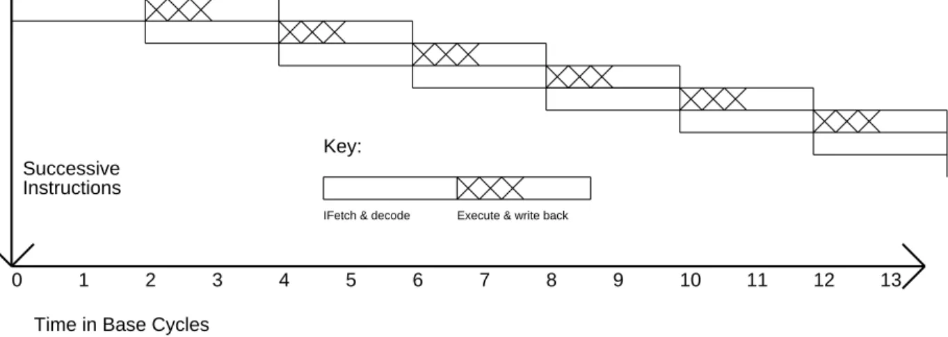
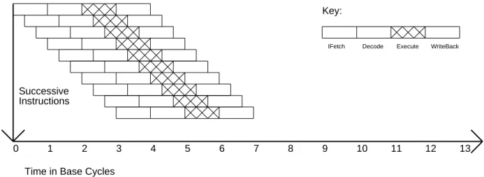
To properly compare performance improvements resulting from the use of instruction-level parallelism, we define a base machine that has an execution pipestage parallelism of exactly one. If instruction-level parallelism of n is not available, delays and dead time will occur when instructions are forced to wait for the results of previous instructions. A second difference is that when the available instruction-level parallelism is less than that which can be exploited by the VLIW engine, the code density of the superscalar engine will be better.
Despite these differences, in terms of runtime utilization of instruction-level parallelism, the superscalar and VLIW will have similar characteristics.
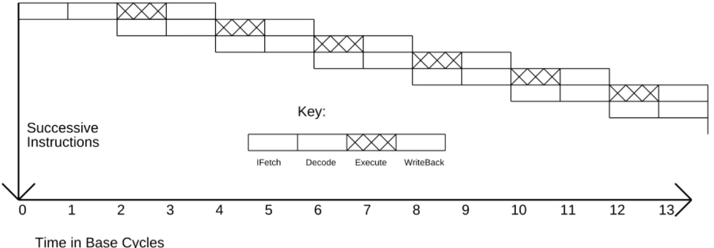
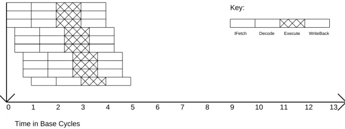
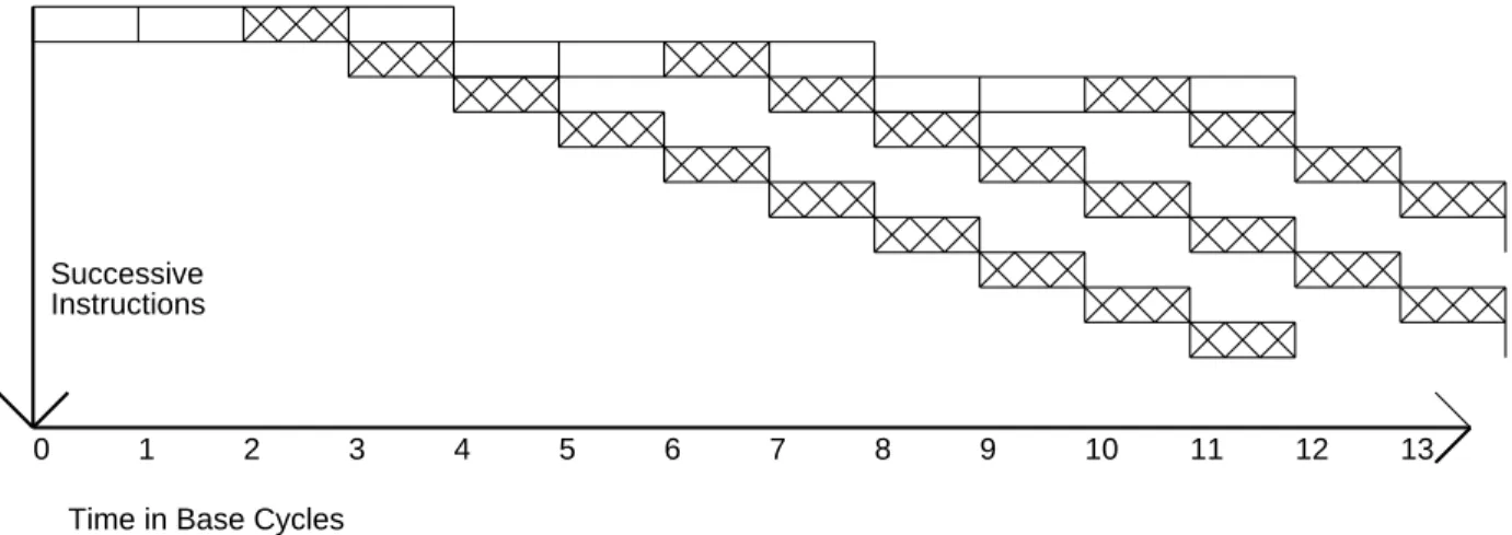
Superpipelined Machines
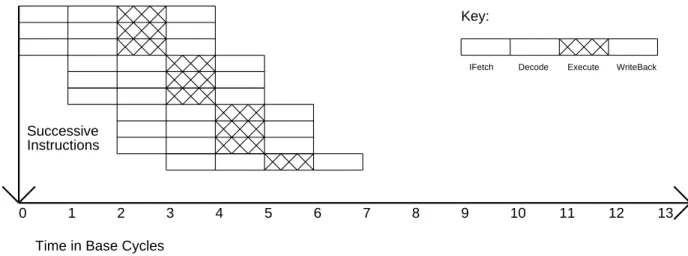
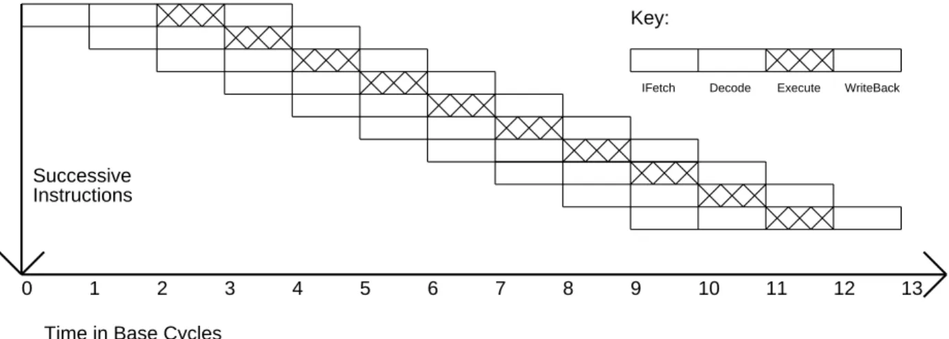
Superpipelined Superscalar Machines
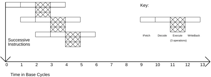
Vector Machines
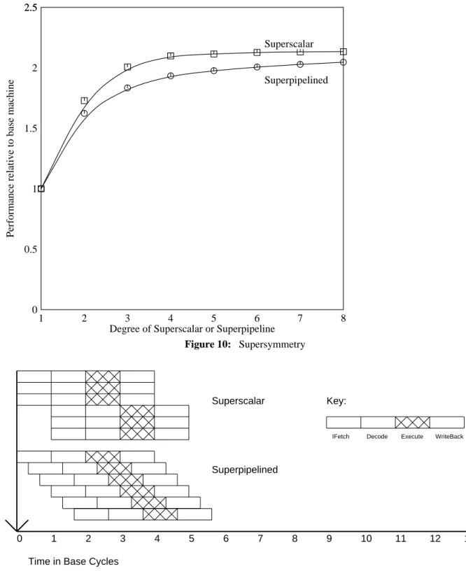
Supersymmetry
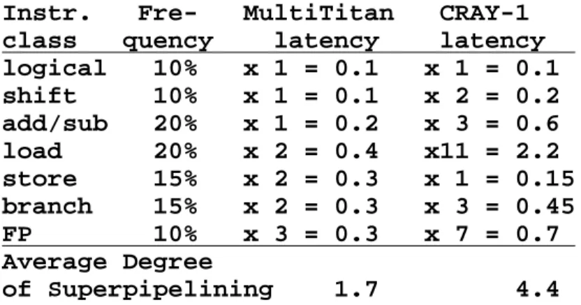
Each of these machines issues instructions at the same rate, so superscalar and superpipe machines of the same degree have essentially the same performance. So far we have assumed that the latency of all operations, or at least simple operations, is one basic machine cycle. For example, few machines have a single load cycle without possible data locking before or after the load.
Consider MultiTitan [9], where ALU operations are one cycle, but loads, stores, and branches are two cycles, and all floating-point operations are three cycles. If we multiply the latency for each instruction class by the rate we observe for that instruction class when executing our benchmark set, we get the average degree of superpipelining. The average degree of superpipelining is calculated in Table 1 for MultiTitan and CRAY-1.
To the extent that some operation delays are greater than one basic machine cycle, the remaining amount of instruction-level parallelism that can be exploited will be reduced. In this case, if the average degree of instruction-level parallelism in the lightly parallel code is around two, the MultiTitan should not stall frequently due to data dependency locks, but data dependency locks should occur frequently on the CRAY. 1.
Machine Evaluation Environment
To specify the pipeline structure and functional units, we need to be able to talk about specific instructions. Therefore, we group the MultiTitan operations into fourteen classes, selected so that operations in a given class are likely to have identical pipeline behavior in each machine. For example, integer addition and subtraction of one class, integer multiplication forms another class, and loading of one word forms a third class.
If an instruction requires the result of a previous instruction, the machine will stall unless the operation latency of the previous instruction has expired. The compile-time pipeline instruction scheduler knows this and schedules the instructions in a basic block so that the resulting stall time will be minimized. We can also group the operations into functional units, and specify an issue latency and multiplicity for each.
For example, suppose we want to issue an instruction associated with a functional unit with issue latency 3 and multiplicity 2. It then issues the instruction on the inactive unit, and that unit cannot issue another instruction until three cycles later. The latency of the issue is independent of the latency of the operation; the former affects later operations with the same functional unit, and the latter affects later instructions that use the result of this one.
Superscalar machines may have an upper limit on the number of instructions that can be issued in the same cycle, regardless of the availability of functional units. If no upper limit is desired, we can set it to the total number of functional units. It uses a part as a temporary for short-term expressions, including values loaded from variables that reside in memory.
It uses the other part as home locations for local and global variables that are used enough to justify keeping them in registers rather than in memory. When the number of operations performed in parallel is large, it becomes important to increase the number of registers used as temporary. This is because using the same temporary register for two different values in the same basic block introduces an artificial dependency that can interfere with pipeline scheduling.
Results
- The Duality of Latency and Parallel Issue
- Limits to Instruction-Level Parallelism
- Variations in Instruction-Level Parallelism
- Effects of Optimizing Compilers
Studies dating back to the late 1960s and early 1970s [14, 15] and continuing today have observed average instruction-level parallelism of about 2 for code without loop decomposition. Since a single-degree (2,2) superpipelined superscalar machine would require an instruction-level parallelism of 4, it seems unlikely that it would ever be worthwhile to build a superpipelined superscalar machine for moderately or slightly parallel code. From this it is clear that large amounts of instruction-level parallelism would be required before issuing multiple instructions per cycle could be guaranteed on the CRAY-1.
In reality, based on Figure 12, we would expect that the performance of the CRAY-1 will benefit very little from parallel instruction is-. We simulated the performance of the CRAY-1, assuming single-cycle latencies of functional units and actual latencies of functional units, and the results are shown in Figure 13. The official version of Linpack has four times the inner loops rolled out and has an instruction level parallelism of 3.2.
We can see that there is a factor of two difference in the amount of instruction-level parallelism available in the different benchmarks, but the upper bound is still quite low. This is largely due to spurious conflicts between different copies of the unwound loop body, which impose a sequential frame for some or all computations. Careful unrolling gives us a more dramatic improvement, but the parallelism available is still limited, even with tenfold unrolling.
The parallelism was 11 for the carefully unwound inner Linpack loop and 22 for one of the carefully unwound Livermore loops. Although we see that moderate loop unwinding can increase instruction-level parallelism, it is dangerous to generalize this claim. These useless calculations give us an artificially high degree of parallelism, but we fill the parallelism with a lie.
If our computation consists of two branches of comparable complexity that can be executed in parallel, then optimizing one branch reduces the parallelism. On the other hand, if the computation contains a bottleneck that other operations are waiting for, then optimizing the bottleneck increases parallelism. We also insert a large calculation before the loop, but if the loop executes many times, changing the parallelism of code outside the loop won't make much difference.
For most programs, further optimization has little effect on instruction-level parallelism (although of course it has a large impact on performance). It turns out that these redundant calculations are not bottlenecks, so removing them reduces parallelism.
Other Important Factors
Cache Performance
Design Complexity and Technology Constraints
First, the added complexity can slow down the machine by adding to the critical path, not only in terms of logical steps, but in terms of the greater distances that must be traveled when passing a more complicated and larger machine. As we've seen from our analysis of the importance of latency, hiding extra complexity by adding extra pipeline stages won't make it go away. Also, the machine can be slowed down by having a fixed source (eg, good circuit designer) spread thinner due to a larger design.
If implementation technologies are fixed early in a design and processor performance quadruples every three years, a year or two of error due to additional complexity can easily negate any additional performance gained from complexity. Since a superpipelined machine and a superscalar machine have roughly the same performance, the decision whether to implement a superscalar or superpipelined machine should be based primarily on their feasibility and cost in different technologies. For example, if a TTL machine were built from off-the-shelf components, designers would not have the freedom to insert pipeline stages wherever they wanted.
For example, they would be required to use multiple multiplier chips in parallel (i.e. superscalar), rather than pipeline a multiplier chip more heavily (i.e. superpipelined). For example, if short cycle times are possible using fast interchip signaling (eg ECL with terminated transmission lines), a superpipelined machine would be possible. In general, if possible, a super-pipelined machine would be preferable, as it only touches existing logic more heavily by adding locks rather than duplicating functional units as in the superscalar machine.
Concluding Comments
The optimization had a larger effect on the parallelism of the numerical benchmarks, but the size and even the direction of the effect depended strongly on the context of the code and the availability of temporary registers. Finally, many machines already take advantage of most of the parallelism available in non-numerical code because they can issue an instruction every cycle but have operation delays greater than one. Thus, for many applications, you should not expect significant performance improvements due to problems with parallel commands or higher pipeline levels.
Acknowledgements
In Second International Conference on Architectural Support for Programming Languages and Operating Systems, pages 100-104.
WRL Research Reports
WRL Technical Notes
List of Tables