compression train system via MINLP optimization

I would also like to thank my best friend and colleague Dj ˆeida Rodrigues for all the friendship and working partnership during these five years of the course. In order to better understand the system, a sensitivity analysis was performed for the CO2 inlet mass flow rate and compression set discharge pressure.

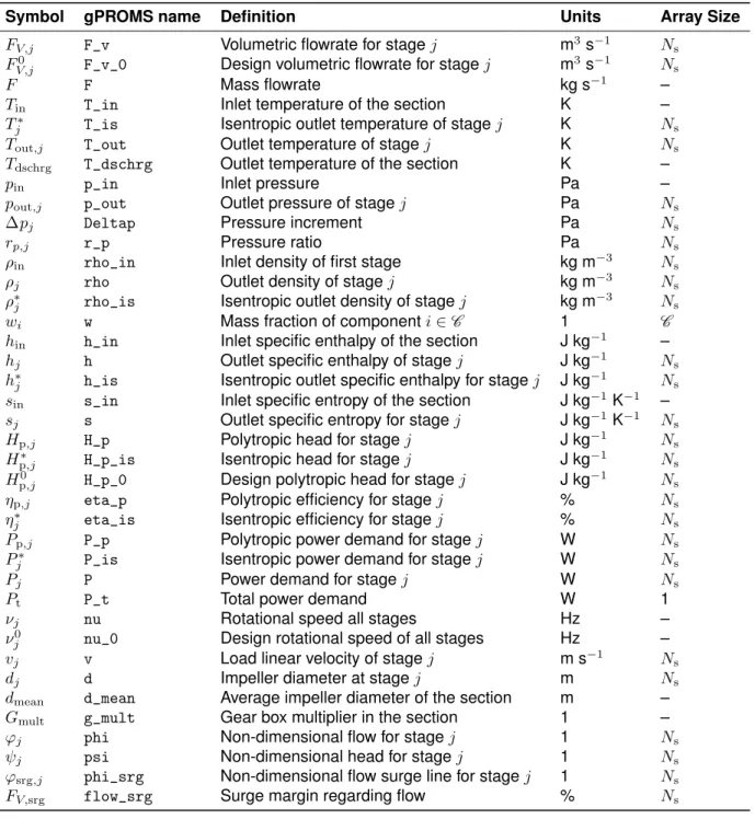
List of Symbols

Introduction

In terms of application areas, the synthesis of heat exchanger networks is one of the best understood and developed, followed by separation systems and reactor networks. In terms of application areas, the synthesis of heat exchanger networks is one of the best understood and developed, followed by separation systems and reactor networks.

Background

Power Plant

A power plant (or power station) is an industrial facility for the generation of electrical energy. This energy can be provided by the combustion of biomass or fossil fuels such as coal, oil, natural gas, or by cleaner and renewable sources such as solar energy, wind energy and hydropower.

Capture Plant

Carbon Capture Technologies
Pre-combustion
Post-combustion
Oxy-combustion

In a gas turbine combined cycle (CCGT) power plant, there are two types of turbines: gas turbines where the flue gas produced by the combustion of natural gas produces some electrical energy provided by its expansion operations, and the usual vapor turbines. The purpose of a post-combustion capture process is to selectively separate CO2 from the remaining gas mixture, so that CO2 can be compressed after the capture facility and stored underground or used in other processes such as Enhanced Oil Recovery (EOR). mass basis) of CO2 in the flue gas produced by coal-fired power plants and 4-5% (molar basis) in the flue gas of natural gas-fired power plants, the capture strategies used in post-combustion typically achieve a CO2 capture efficiency of 90% [ 4 ].

Compression Train System

Work of Compression
A Adiabatic (or isentropic) compression
B Isothermal compression
C Polytropic compression
Multi-stage Compression with Intercooling
Compressor
Electric Drive
Cooler and Knock-out Drum
Dehydrator

Normal air cooling can be used to reduce the temperature of the CO2 stream from 140oC to 35oC. 2.4) Whereρ2is the density of the outlet current corresponding to the inlet entropy (isentropic process). Due to the high flow rate of the CO2 stream involved in the CCS process, centrifugal compressors are preferred over reciprocating compressors in most cases.

With the correct pore size, water will be adsorbed into the molecular sieves of the dehydrator, allowing CO2 to flow to downstream equipment.

Pipeline and Transportation

Dehydration at higher pressure requires a smaller and cheaper dehydration system because upstream compression and intercooling remove some of the water from the CO2 stream. Increasing the exhaust temperature will result in a reduction in the efficiency of the compression system, resulting in higher operating costs due to higher energy consumption. Another advantage of locating the dehydration system near the first compressors is the reduction of the metallurgy costs of the entire compression system.

The part of the compression system upstream of the dehydration system must be constructed of expensive duplex stainless steel (because the corrosion is caused by the wet CO2), the downstream equipment need only be constructed of carbon steel (which is cheaper). .

Injection and Storage

Injection
Storage

At the bottom of the injection site, CO2 is dispersed, leaving a trace of trapped CO2 (in light purple) as bubbles in the pores. CO2 also dissolves in the brine (in blue) and slowly sinks through the aquifer (in light blue) because it becomes denser than brine [22]. The geological storage of CO2 can be undertaken in a variety of geological environments such as basins, oil fields, depleted gas fields, deep coal seams and salt formations which are represented in figure 2.29.

In cases where CO2 is not soluble in oil, injection of CO2 increases reservoir pressure, which helps sweep and push oil toward the production well [24].

Materials and Methods

The parameters can be defined as integers, real or foreign objects (such as the performance maps of the compressors). Variable types represent a separate entity in ModelBuilder, and both limits and default value must be defined in the VariableTypesection. To connect the different component models in a topology environment, a port connection must be defined in the ConnectionTypesection and added to the models.

These model types have the same structure as the previous ones, but the component models that use them must be defined in the Unit section.

Model development workflow

Compression System Component Models Description

CompressorSection

In performance (off-design mode), gas flow rate is related to device head, suction conditions, compressor speed, and performance characteristic maps. Option 1a: User-defined one-dimensional performance maps at a specified rated speed; the model uses affinity laws to determine performance at other speeds. In design mode (option 3), inlet conditions and outlet pressure are specified by the user, and the number of stages, rotor diameter, and stage performance maps are generated by external code associated with the model.

ElectricDrive

The Electric Drive model is connected to the first compressor section, transmitting the engine speed to it, but receiving the necessary power from all compressors belonging to the same frame. This model also warns the user when the total power required exceeds the maximum power (design power). In the second option, the mechanical efficiency is calculated based on the load fraction, i.e. the ratio of operating power to design power.

In VFD mode, electrical efficiency must be considered, introducing an electrical efficiency specification to calculate the real electrical energy demand.

CoolerKODrum utility

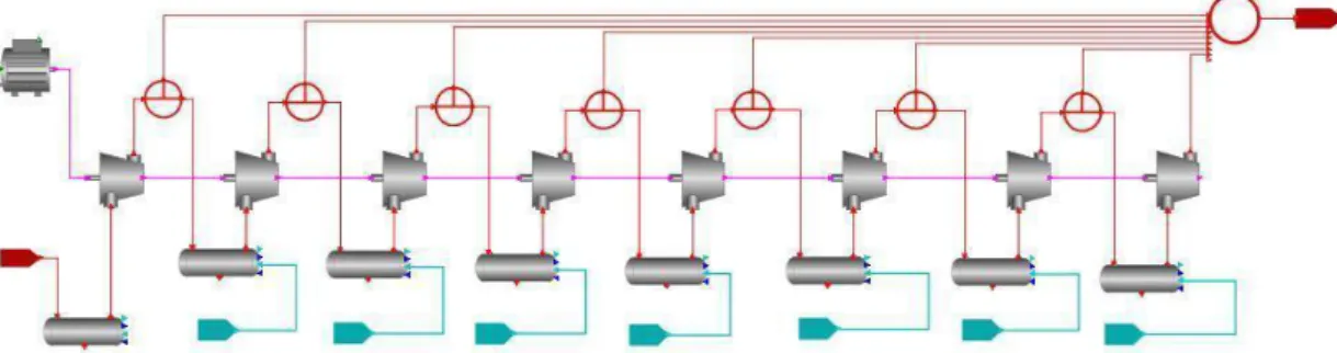
Modeling of a Compression Train System

Flowsheet Implementation

At the outlet of the cooler, the LP flow is mixed with the MP flow coming from the AGR and at 1oC with a CO2 volume concentration of 97.3%. This dehydration unit is a three-bed absorber, described in section 2.3.6, where the regeneration of the saturated bed is carried out using a portion of the dried gas product (typically about 10%). The flow used for regeneration is then returned to the outlet of the final compression stage before the dehydrator.

Where M represents an electric drive and frames 1, 2 and 3 represent the different compression frames of the compression train.

Simulation Results

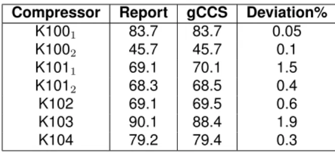
The CO2 stream is then directed to a dehydration which is sized to reduce the water content of the CO2 stream to 50 ppmv in accordance with the typical transmission grid specification. Note that between the third and fourth stages of compressor K100 and the second and third stages of compressor K101 there is an intercooler that cools the CO2 stream to 19oC. This explains the accuracy of the simulation results compared to the report data from [27].

Due to the complexity of this problem, only the first half of the train was considered in this work.

Optimization Problem Formulation

MINLP Formulation
Objective Function and Cost Estimation

Objective Function
Cost Estimation of CAPEX and OPEX

Superstructure
Simplifications and Assumptions

Note that due to the linearization of the non-convex functions, there is no guarantee of finding the global optimum. Further analysis of the number of degrees of freedom (DOF) will be done in the next sections. Another reason for this simplification is that optimizing the number of steps per section would exponentially increase the complexity of the MINLP.

In this formulation, the unknown variables are the pressure ratio of each compressor (assuming they all have the same value) and the eight binary variables of zk (where their sum must be 1), so the number of DOF of the system is eight.

Optimization Results

Point Optimization

Initial train optimization
Pressure ratio profile
Drive speed

Intercooling Decision
Sensitivity Analysis

CO 2 flowrate
Discharge pressure

Multi-period Optimization

Problem formulation
Comparison against previous design strategy

Analyzing figure 7.5(a), it is possible to observe that the optimal number of compressors for the new formulation is 5 instead of the 4 compressor train given by the previous formulation. The function between total cost of the optimal train and the speed (figure 7.8) is almost linear and does not have a minimum. In this section, a sensitivity analysis was performed for the inlet CO2 flow rate and final discharge pressure of the train using the same methodology used for the speed drive.

Increasing the CO2 discharge pressure also increases the number of compressors in the optimal train from 5 to 6.

Conclusions and Future Work

Conclusions

Knowing the influence of the volume flow rate on the efficiency of the compressor, the optimization problem was reformulated and the pressure ratio was optimized for each specific compressor section. The results were clear as the balance of compression work done by the new formulation resulted in a reduction in total cost and the optimal train configuration changed from 4 to 5 compressors. In order to gain a better understanding of the system, some assumption tests and sensitivity analyzes were performed.

The behavior of the system and the changes in the optimal train configuration were also analyzed for the key process variables.

Future Work

The implementation of the entire compression train, the incorporation of a better cost model and the integration of the number of steps optimization are pointed out have the most important key aspects that need to be improved in this work in the future, since with these changes this tool can become very similar to the final version of a true self-configurable compression train system. By combining two sets of the superstructure implemented in this work with a dehydrator model between them, the total cost can be minimized and the effect of all decision variables taken into account, such as the number of compressors before and after the dehydrator, pressure ratio of all compressors or the recycle flow from the dehydrator , can be analyzed and quantified. Adding a condensing unit and CO2 pump models to the flowsheet (already available in the gCCS library) will allow a process synthesis of the new CO2 liquefaction superstructure to be performed.

After the technology area of compression system synthesis has been developed, the possibility of combining the optimization of the train with other CCS chain components becomes a reality.

Bibliography

Metz, "Carbon Dioxide Capture and Storage: Underground Geological Storage,"Intergovernmental Panel on Climate Change, 231, 2005. Metz, "Carbon Dioxide Capture and Storage: Underground Geological Storage,"Intergovernmental Panel on Climate Change, 199, 2005. 35] Floudas og Paules, "A Mixed-Integer Non-linear Programming Formulation for the Synthesis of Heat Integrated Destillation Sequence,"Computers and Chemical Engineering, 1988.

Metz en et al., “Carbon Dioxide Capture and Storage: Carbon Dioxide Transport, Injection and Geological Storage”, Intergouvernementeel Panel over klimaatverandering.

CompressorSection

Model assumptions
Nomenclature
Ports
Equations

Hj1D(ϕ) interpolatie_1D_phi_psi 1-D dimensional map FO – Ns Ej1D(ϕ) interpolatie_1D_phi_eta 1-D dimensional map FO – Ns.

Performance mode equations

Ns (A.48) Design head, flow rate, ϕ and ψ are not needed in this mode, so set them to zero:.

Port connections

Performance map generation

By assuming a value of the flow coefficient phi that leads to the maximum efficiency in Figure A.1(a), the design phi is determined and the diameter can also be calculated based on the inlet conditions and the compressor speed. Using the design efficiency and pressure ratio, the polytropic head and design head coefficient can be calculated. Now that the design flow coefficient, head coefficient and efficiency have been determined, the performance maps are generated using a generic normalized map.

So, to generate the performance maps, the normalized maps must be multiplied by the design point.