Coupled Aircraft Design and Trajectory Optimization of an Electric UAV

A ferramenta foi adaptada para permitir a propulsão elétrica e calcular parâmetros de desempenho relevantes, bem como o componente de trajetória, que é implementado através de um método de posicionamento. A otimização é realizada utilizando um método gradiente para diversos objetivos, como minimizar a energia consumida durante a fase de subida, minimizar o tempo de subida até uma determinada altitude e maximizar o alcance a partir de uma fase de cruzeiro do voo.

Motivation

Whatever the objective, the aircraft itself can be improved by any of the various engineering disciplines involved, such as the propulsion system, aerodynamics and structures. This part of the mission optimization is usually done post-design, so it is limited by the capabilities of the aircraft.

Aircraft Design and Trajectory Optimization

Manufacturers usually create new products as iterations of proven concepts, but with changes that improve certain features of the previous model. In the case of commercial aircraft, for example, this is usually to reduce fuel consumption as a way to increase profits.

Objectives and Deliverables

Thesis Outline

Aircraft Geometry

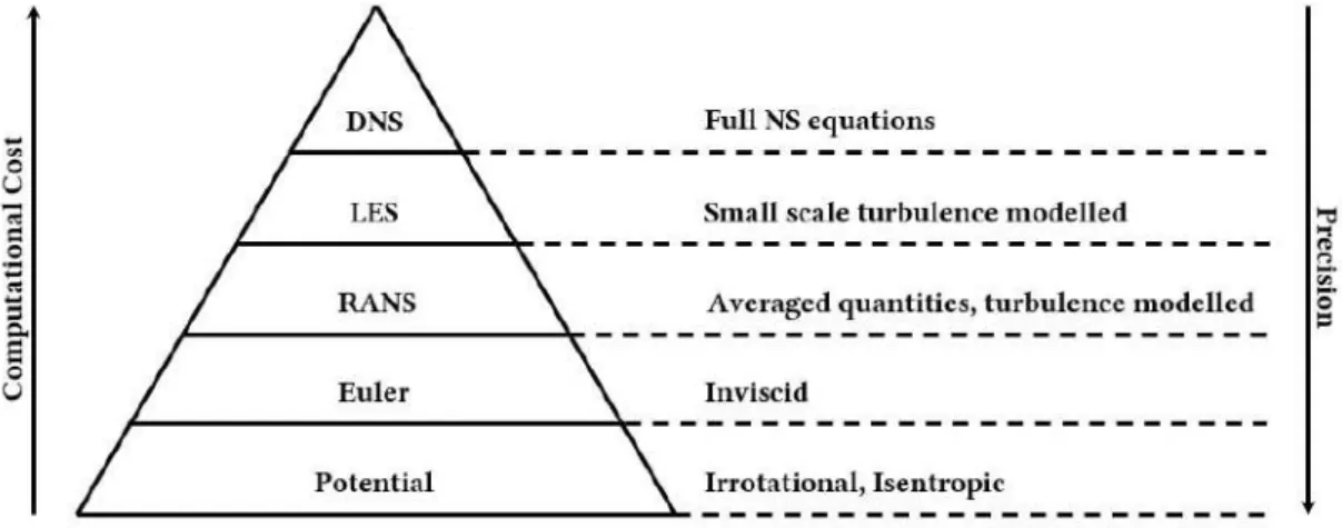
This chapter presents models of analytical disciplines and their theoretical background. The pipe can be placed on any part of the chord and this position limits the maximum diameter per heightℎsection.

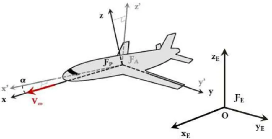
Aircraft Dynamics

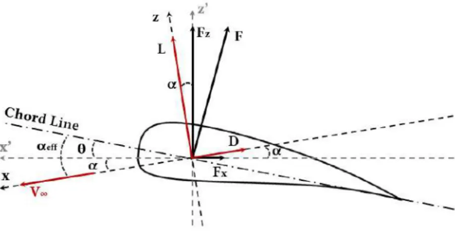
These simplifications are shown in Figures 2.4(a) and 2.4(b), respectively. a) Representation of the forces acting on the center of mass of the aircraft. The derivation of the equations of motion is done in the flight path frame and in the earth frame.

Aerodynamic Model

In other words, the velocity induced at the control point 𝑘 due to the panel 𝑗 is the sum of the contributions of the strands, . 2.7, is the effective angle of attack that the air velocity makes with the chord line of the section containing the panel.

Structural Model

The complete stiffness matrix for an element is obtained by superimposing the stiffness matrices of the individual elements, yielding. The spar considered here has a circular cross-section. where 𝜎 and 𝜏 represent normal and shear stresses, respectively, the subscript 𝑖 is the axis𝑦or𝑧and 𝑟 is the radius of the tube, the point of maximum stress. 2.12(a), the yield stress is the limit of the elastic behavior of the material, therefore the equivalent stress must be lower than the yield stress to avoid plastic deformation.

Propulsion Model

• Battery
• Motor
• Propeller
• Propulsive System

In this work, the energy density of the battery is considered to be 210 Wh/Kg, a value within the range of Li/ion and Li-Po batteries. The rate of rotationΩ is related to the electromotive force (EMF), 𝑣𝑚, by means of the speed constant. and the EMF can be obtained by solving the circuit's equation, according to Kirchhoff's voltage law. where𝑅 is the motor's resistance. The performance of the propeller is usually described with Blade Element and Momentum Theory, which is the basis of the relationship used in this work to calculate the thrust.

Aircraft Design and Control

A full description of the theory and derivation of the equation is given in [29]. 𝑠𝑘is the area of ​​the propeller disk. The combination of the propulsion component models described earlier results in the propulsion system algorithm. Two structural constraints are imposed to prevent failure of the wing shoulders and tail, which is achieved through the Von Mises yield criterion.

Aircraft Performance and Operating Point

Trajectory Optimal Control

This chapter begins by presenting the formulation of the optimal control problem, followed by an example of a one-dimensional trajectory problem, which is later used to illustrate and compare the differences between direct recording and collocation transcription methods. Numerical methods for solving optimal control problems are divided into three main methods: dynamic programming, indirect methods and direct methods. Regarding indirect and direct methods, Rao [36] explains that a well-founded optimal control problem has two of the three main components at its core (Table 3.1).

Indirect Methods

This is the basic principle of the calculus of variations used in the derivation of the necessary conditions of optimality. To illustrate the derivation of the first order necessary conditions, let us consider a problem similar to that in Eq. The first step of the derivation is to write the Lagrangian of the objective function.

Direct Methods

Direct Shooting

Indirect methods are very accurate, but their applicability is limited because they require an analytical derivation of the necessary first-order conditions for each new problem [37]. Due to the nature of the firing methods, NLP does not have an explicit dynamic constraint, which does not mean that the dynamics will not be met. As Betts [32] noted, shooting methods face some problems related to the sensitivity of the variables.

Direct Collocation

Pseudospectral (or global orthogonal) collocation methods are a class in which the parameterization of the state and control is performed using global polynomials. Compared to shooting methods, collocation has the advantage that the computationally expensive numerical integration of the differential equations can be avoided [41]. Using this collocation method with the same grid size, the number of variables is triple that of the shooting method and the constraints almost double.

Trajectory Design and Control

Problem Statement

However, aerodynamic and structural constraints must be met throughout flight and the aerostructural system is solved to obtain the forces required for the equations of motion.

Multidisciplinary Analysis

As a result, the system equation𝐴𝑥 = 𝑏can be solved for𝑥𝑖 45] compare Coupled Newton (CN) and Nonlinear Block Gauss-Seidel (NLBGS) with Aitken relaxation for a scaling problem with total tunable number of variables, degree of nonlinearity, joint strength and sparse structure. It can be seen that the strongly coupled problems take longer to converge for all solvers, except for NLBGS without Aitken relaxation, which does not converge at all.

Multidisciplinary Design Optimization

In the aerostructural problem, it increases with the load factor and with the decrease in beam thickness. This is desirable, because if the optimization is terminated prematurely, there is a physically feasible design point [50]. However, this does not mean that the design constraints are necessarily met, as this depends on whether the optimization algorithm maintains a feasible design point [47].

Optimization Algorithms

Defining the Lagrange function as. 4.17) is its derivative with respect to 𝒙 and the optimality conditions can be expressed in Lagrangian terms as Given the advantage of gradient-based methods and the good performance of the open-source SLSQP, this is the algorithm used in this work. The total sensitivity of 𝑓 is given by. and the total derivative of the governing equation is . Partial derivatives can be easily calculated by changing the denominator and re-evaluating the numerator, but total derivatives require multidisciplinary problem solving.

Aerostructural Analysis and Optimization Tool

The equivalent nodal force and moment at one of the structural nodes is given by. These equations immediately satisfy the consistency requirement, since they are equivalent results of the aerodynamic load distribution. The virtual work on the aerodynamic mesh is written as. where the displacements are given by. 4.43) With this we conclude that𝛿𝑊𝑎= 𝛿𝑊𝑠and the transfer scheme is conservative.

Framework Implementation

The energies of all mission points calculated in the drive are summed in the mission capacity to give the total energy consumed and the energy limit value. Then the sum of the forces and energy expended at each point is passed to mission_perf. Here, the energies are added together to get the total energy used and the energy limit value.

Baseline Problem Definition

Solver and Optimizer Parameters

The optimization is first performed for the three problems previously defined (DP, TP and DTP) with the aim of minimizing energy.

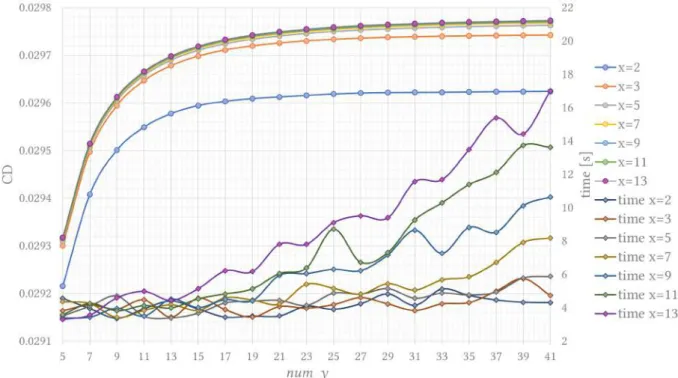
Mesh Convergence Study

The mesh of each lifting surface is defined by the number of nodes in the chord and span directions, num_x and num_y respectively. It can be seen that increasing the number of panels gives larger 𝐶𝐷up to a certain point where it starts to stabilize. Therefore, the number of panels for the wing is 6 × 30, while for the tail a panel ratio of 3 is given.

Aircraft Configuration

The center of mass of the aircraft without lifting surfaces, referred to as empty CG, is assumed to be 0.2 m forward of the trailing edge of the wing. Based on the information that the maximum take-off weight of the AR4 is 4 kg, the empty mass is assumed to be 1.2 kg and the battery mass is 1.5 kg. The spar is placed at 30% of the chord on both surfaces, which is the point where the thickness to the chord ratio (ℎ/𝑐) of the airfoil is greatest.

Optimal Design for Minimum Energy Climb

Baseline Trajectory

Results

The Hessian measures are given by the square of the sum of design variables and constraints. This was achieved by reducing the thickness of the spars and the size of the lifting surfaces. The only other factor these angles affect is the length of the beam.

Optimal Design for Minimum Time Climb

As lift increases with speed and angle of attack up to stall, yaw tends to decrease values ​​in the time minimization problem, yielding a lower effective angle of attack as a way to compensate for the. Since lift was almost the same, the stabilizer angles required to trim the aircraft were also similar, as seen in Fig. As a result, efficiency increases with speed, which explains why it was higher in the time minimization problem.

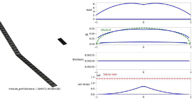
Optimal Design for Maximum Range

Despite the large aspect ratio, stresses had good margin to the failure limit, as seen in Fig. As previously stated, most of the energy was used in horizontal motion rather than vertical. We see that the first half of the flight was almost horizontal, with flight path angles lower than -0.1°.

Summary

This decline coincides with the beginning of the steeper decline phase, as the output thrust was no longer sufficient to maintain equilibrium of forces. Keeping this in mind, battery capacity is one of the limiting factors of this problem. This was the result of the low thrust and high angle of attack, because for a fixed velocity, lower thrust increases efficiency, and similarly, higher angles of attack decrease perpendicular velocity, thus increasing thrust and efficiency.

Achievements

Future Work

On the dynamical theory of incompressible viscous fluids and the determination of the criterion. A review of three pseudospectral methods for the numerical solution of optimal control problems. Neyman, editor, Proceedings of Second Berkeley Symposium on Mathematical Statistics and Probability, pages 481–493.