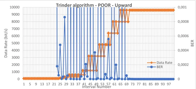
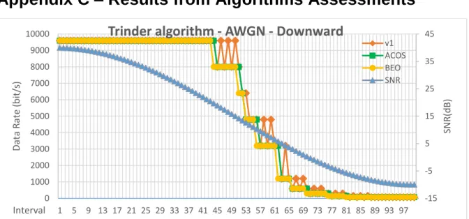
70 Figure C.1 – Data rate adjustment of Trinder algorithm for AWGN channel using downward sine variation of SNR. 79 Figure C.4 – Trinder algorithm data rate adjustment for AWGN channel using SNR upward sine variation.
Introduction
- Context and Motivation
- Objectives
- Main Contributions
- Dissertation Structure
To deal with HF channel variability, several technologies have emerged, such as automatic Link Quality Analysis (LQA), Automatic Link Establishment (ALE), and automatic Data Rate Change (DRC), which eliminate the need for complex and manual operating procedures [2]. As mentioned before, in the early 2000s some algorithms were developed to improve HF communication efficiency, the main topic of this thesis.
![Figure 1.2 – Image of the E/R GRC-525 [2].](https://thumb-eu.123doks.com/thumbv2/123dok_br/19768780.0/24.892.329.558.424.575/figure-1-2-image-e-r-grc-525.webp)
HF Communications
Types of HF Radio Signals
Propagation by the Ionosphere
- The Ionosphere Layer
- Near-Vertical Incidence Sky wave
This sky wave uses high tilt angles (between 60º and 89º) and the Ionosphere to reflect signals back to Earth. There are three important factors to consider in NVIS communications: interference between the Earth wave and the Sky wave, high tilt angles, and critical frequency selection.
![Figure 2.3 – Ionosphere behaviour: a) reflection depending on the frequency; b) reflection depending on the day time [13]](https://thumb-eu.123doks.com/thumbv2/123dok_br/19768780.0/29.892.156.743.238.503/figure-ionosphere-behaviour-reflection-depending-frequency-reflection-depending.webp)
HF Antennas
One of the methods to improve the efficiency of the Whip antenna is to place the antenna at an angle of 45º to the vertical axis of the vehicle, which transforms the Whip into a nearly horizontal dipole antenna [16]; When working in NVIS, there is no need to be concerned about the orientation of the dipole antenna, as all energy is propagated in the vertical direction and returns to Earth with an omnidirectional "umbrella" shape diagram.
HF Communication Standards
- Adaptive Techniques in HF Communications
- Overview of HF Communications Standards
- Physical Layer
- Automatic Channel Selection (ACS)
- Automatic Link Establishment (ALE)
- Automatic Link Maintenance (ALM)
- Data Link Protocol
- High Throughput Data Link
- Low Latency Data Link
- High Throughput Data Link+
The main vulnerability discovered by combining the analysis of the data rate adaptation (in Figure 5.8), the link availability results (in Table 5.1) and the BER versus data rate variation (in Figure 5.9) is the data rate oscillations that lead to many cut-off states, which reduces the link's availability. The connection distance is 282 km, with Station 1 located in Logistics Support Unity, Paço de Arcos, Lisbon and Station 2 located in Signal Regiment, Viso de Baixo, Porto; .. the location of the stations is represented in Figure 6.11, provided by Google Maps. a) b).
![Figure 3.1 – ARCS process cycle [18].](https://thumb-eu.123doks.com/thumbv2/123dok_br/19768780.0/36.892.372.544.103.275/figure-3-1-arcs-process-cycle-18.webp)
State-of-the-art on Data Rate Change Algorithms
DRC algorithm for non-Autobaud Modulations
Trinder and Brown proposed in [30] one of the first DRC algorithms; the main task of the algorithm was to serve as a guideline for implementers of STANAG 5066. Another problem with the algorithm involves the time required to obtain enough data to estimate the FER with precision.
DRC algorithm for Autobaud Modulations
This effect is particularly prevalent in an AWGN channel, which has very abrupt BER curves and thus causes a very sharp change in FER values, even with an almost constant SNR [3]. Therefore, it may take a long time to perform data rate adaptation, losing efficiency. The 2400 bit/s data rate is never used in this algorithm, the transition between Autobaud and non-Autobaud modulations is between the 3200 and 1200 bit/s data rate values.
Nieto [31] evaluated DRC algorithm for Autobaud modulations using different packet sizes and varying SNR values, over three types of channels: ITU Poor, ITU Good and AWGN channel. Nieto also indicated that the development of a DRC algorithm is quite complex due to the large number of variables involved such as the message size, frame size, current channel conditions including SNR and BER, available modem data rates and interleaver size. Use the long and short interleaver for common channels, and the long one for faded channels.
The choice of which interleaver to use is a trade-off between the delay due to interleaver delay and the reduced FER. Based on the analysis presented in [6], Trinder and Gillespie recommended that a shorter interleaver should always be used, except in the broadcast data exchange mode where a long interleaver is preferred.
RapidM DRC algorithm
- RapidM DRC algorithm 1 design
- RapidM DRC algorithm 1 implementation
- RapidM DRC algorithm 1 simulation, results and tests
DRC Algorithm: Assessment of Existing Solutions and Proposals for Improvement
DRC Algorithms Simulation System
It is worth noting that (5.1) is only an approximation of BER vs SNR, valid for the range of BER values showing a linear variation with SNR, in logarithmic units; as shown in Figure 5.2, for BER. This process shown in Figure 5.3 is only used in the TX station because the transmitted frame has a header with the current data rate and after the RX station reads the header, it will update this data rate. Average data rate (in bit/s) – defined by (5.3), where 𝐷𝑅𝑖 is the data rate value for the slot number 𝑖, 𝑇𝑖 is the duration of the slot and 𝑁 is the total number of slots.
Average BER – defined by (5.5), where 𝐵𝐸𝑅𝑖 is the calculated BER value for the slot number 𝑖. Whenever the BER value is higher than 10−3, it is considered that the link is in a down state; an auxiliary variable, 𝜏𝑖, calculated from (5.4), accounts for the time intervals that are not in the cutoff state. Average flow (in bits/s) – defined by (5.8), represents the number of correct bits/s at the receiver.
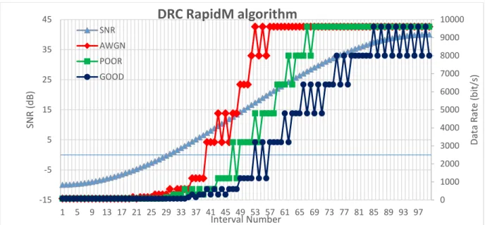
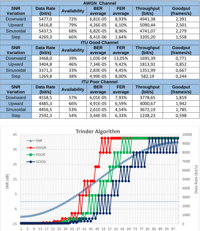
Average good feedback (in frames/s) – defined by (5.9), where 𝐿 is the frame length in bits, represents the number of correct frames/s at the receiver. To assess the algorithms, four types of channel SNR variations were considered: downward sinusoidal, defined by (5.10) and represented in Figure 5.4; upwardly sinusoidal, defined by (5.11) and represented in Figure 5.5; sinusoidal, defined by (5.12) and represented in Figure 5.6; and stepwise, represented in Figure 5.7 and whose behavior is closest to a real channel.
![Figure 5.2 – BER as a function of SNR for m-QAM modulation, with a straight line (in green) representing a BER variation of 1 decade per dB (Adapted from [32])](https://thumb-eu.123doks.com/thumbv2/123dok_br/19768780.0/56.892.235.668.223.586/figure-function-modulation-straight-representing-variation-decade-adapted.webp)
Previous DRC algorithms: Simulation and Assessment
- Trinder algorithm Simulation and Assessment
- RapidM DRC algorithm Simulation and Assessment
The RapidM DRC algorithm bases the data rate decision in four rules: the first two rules calculate the next data rate based on SNR variations; the third rule performs data rate decisions based on the calculated BER value, as in the Trinder algorithm; and the fourth is a safety rule that allows the data rate to increase by at most two steps at once and to decrease by three steps at once. The link assessment results are represented in Table 5.2 for the three considered channel types; Figure 5.10 shows the data rate variation for the considered channels and for an upward sinusoidal SNR variation. The same proposal to improve link quality for the Trinder algorithm will also be considered for the RapidM algorithm; if the new data rate leads to cut-off condition, the previous data rate will be maintained.
The relative variation of these assessment metrics is represented in Table 5.3 and calculated using (5.20), where x is the percent relative variation, obj is the RapidM algorithm metric value, and ref is the reference value (obtained using the Trinder algorithm).
Improvements on the Trinder and RapidM Algorithms
- Avoiding Cut-Off State Algorithm
- Bit Error Optimization Algorithm
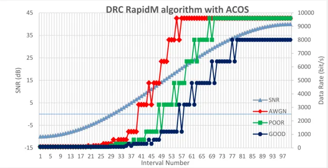
The link data rate variation for the Trinder algorithm with ACOS is represented in Figure 5.13 (for an upward sinusoidal SNR variation); Table 5.4 presents the assessment metric values, and Table 5.5 presents the relative variation between both algorithms. A graphical comparison between Trinder algorithm with ACOS and the original version is presented in Appendix C. The vulnerability detected in the Trinder algorithm with ACOS was the unnecessary oscillations in each data rate value that can be visualized in Figure 5.14, represented by the BER values higher than 10-4.
The performance of the RapidM DRC algorithm with ACOS is much better than the original version of the RapidM DRC algorithm, as can be seen in Table 5.7, which presents the relative difference between them. The performance results of the Trinder algorithm with BEO are presented in Table 5.8 and Figure 5.18 (for upward sinusoidal variation of SNR) for the three types of channels considered. You can check Appendix C for a comparison of data transfer rates between all versions of the Trinder algorithm; the relative difference between the Trinder algorithm with BEO and the original version is presented in Table 5.9.
The performance results of the RapidM algorithm with BEO are represented in Table 5.10 and Figure 5.20 (for an upward sinusoidal channel) for the three types of channels. The relative variation between the RapidM algorithm with BEO and the original version is represented in Table 5.11, and Figure 5.21 shows how the BER is kept below the BER threshold of the RapidM DRC algorithm.

Conclusion
Field Propagation Tests
- Equipment Assembly and Configuration Procedures
- General Settings and Components
- Assembly of Bench Tests Circuit
- Assembly of Field Tests Equipment
- Data Rate Change Software Application
- User Application Configuration
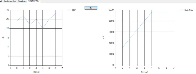
- Output Files and Graphical Views
- Field Propagation Tests: Environment Conditions and Results
- Meteorological and Ionospheric Conditions for Test Days
- Algorithms Performance in Real Test Conditions
- Relation between Simulations and Field Propagation Values
In Figure 6.2, the white line corresponds to the expected value on August 28, 2017, and the red line corresponds to the actual values measured by ionosondes. The ATU process is initialized through the radio menu as shown in Figure 6.6 a); .. if the tuning failed, the following message will appear on the screen: "ANTENNA TUNE FAILED". It was necessary to place a fixed attenuator at the output of the portable terminal as shown in Figure 6.8 b) to avoid large power spikes that could damage the equipment.
The interleaver size should also be selected on this tab, as shown in Figure 6.14. The entire configuration process in the Algorithms tab is shown in Figure 6.15, which represents the data sending settings. Once you have the file, you can send it in the Send File section by filling in the file directory field and pressing the Send button, as shown in Figure 6.16 b).
The cross-correlation coefficients are shown in Table 6.3 for each algorithm tested on different days, and the corresponding plot in Figure 6.24. According to the cross-correlation coefficient values shown in Figure 6.24 and Table 6.3, the field propagation results tend to approximately match the expected results provided by the simulation system.
![Figure 6.2 – Critical frequency of F2 layer in real time for the 28 th of August 2017 (Consulted on [17])](https://thumb-eu.123doks.com/thumbv2/123dok_br/19768780.0/76.892.295.617.422.684/figure-critical-frequency-layer-real-time-august-consulted.webp)
Summary and Future Work
Summary
7 September 2017) coincided with the highest number of ionospheric warnings and the worst average SNR value (3.38 dB). However, the Trinder algorithm with BEO outperformed its original version, increasing productivity by 189% and connection availability by 13%. The original version of the Trinder algorithm presented the worst performance results among any algorithm tested.
Future Work
Gillespie, “Optimization of the STANAG 5066 ARQ Protocol to Support High Data Rate HF Communications,” in Proceedings of IEEE Military Communications Conference (MILCOM) 2001, Washington, DC, October 2001. Brown, Algorithms for Data Rate Adjustment using STANAG 5066, London, UK: IEE Colloquium on Frequency Selection and Management Techniques, 1999. Nieto, An investigation of Throughput Performance for STANAG 5066 High Data Rate HF Waveforms, Anaheim, CA: Proceedings of IEEE MILCOM 2002, 2002.
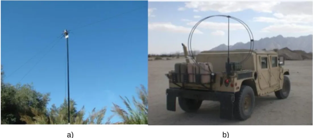
![Figure 2.10 – Antennas used in NVIS: a) horizontal dipole antenna [15]; b) circular loop antenna [21]](https://thumb-eu.123doks.com/thumbv2/123dok_br/19768780.0/33.892.255.637.703.946/figure-antennas-nvis-horizontal-dipole-antenna-circular-antenna.webp)