Development of a Framework for Static Aeroelastic Analysis of Flexible Wings including Viscous Flow Effects

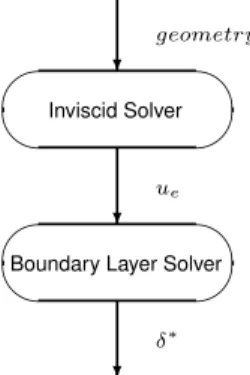
I would also like to thank Jos ´e Fernandes for all his support in the later stages of the development of this thesis. The thickness of the boundary layer is then taken into account in the recalculation of the inviscid flow.

Nomenclature

C] Damping Coefficient Matrix [F] Generalized Force Vector [M] Mass Coefficient Matrix [M] Stiffness Coefficient Matrix q Fluid Velocity Vector CD Drag Coefficient.

Introduction

Motivation

Nowadays, the field of Computational Aeroelasticity (CAE) is in charge of predicting such effects. This work attempts to fill that gap by including the effects of the presence of a boundary layer on a low-fidelity aerodynamic inviscid model.

Objectives

Thesis Outline

With the verifications made, the final solution to the Static Aeroelastic problem previously defined is subsequently obtained from the Aeroelastic Framework, both for an Inviscid and Viscous flow assumption. The results are commented and the effects added by the presence of the boundary layer are evaluated.

Aeroelasticity

Introduction

Aeroelasticity is today a well-established field that deals with the study of the interaction between three forces: aerodynamic, inertial and elastic [10]. As a composite of several disciplines, the formulation of the aeroelastic problem requires inputs from the involved fields.

Aeroelastic phenomena

However, one of the first considerations that must be made within the framework of structural design is static aeroelastic phenomena. Before studying the dynamic aeroelastic phenomena, it is important to determine the static characteristics of the aircraft during these phases.

Computational Aeroelasticity

• Interaction methods
• Interface models
• Fluid models
• Structural models

This section provides an overview of the field of computational aeroelasticity with an emphasis on static aeroelastic modeling. In this way, an iterative process can be used to update the two models, which become equivalent as the calculations progress. Although this avoids an iterative process between aerodynamic and structural solutions, the size of the problems is limited to relatively small ones that are used only in 2D cases.

Commercially available software packages such as ZEUS use an Euler equation solver for the inviscid part of the flow along with a steady boundary layer equation to include viscous effects.

Aerodynamic models

Introduction

By replacing equation 3.3 with 3.2, the Navier-Stokes equations (3.4) are obtained. i, which proves the equilibrium between the fluid acceleration terms on the left and the forces exerted in the fluid. All equations presented in this section provide physical models of flow classes that, under the right conditions, are completely sufficient to obtain an accurate representation of the flow. Numerous versions of the Navier-Stokes equations have also been used recently (included here are the time-averaged Reynolds equations discussed in Chapter 10).

This improves the computational efficiency of the developed code, while not rejecting all the effects of viscosity.

Inviscid flow

• Governing Equations
• Basic flow solutions
• Panel Methods

Making the same assumption of the inviscid flow of an incompressible fluid, the Euler momentum equation (3.12) can be obtained as follows. Taking equation 3.19 and introducing the discretization of the surface into panels gives equation (3.22). The calculation of the frictional resistance will be explained in the following paragraphs with regard to the viscous flow models used.

Determine the Influence coefficient expressions that describe the influence of each panel's singularity distribution in the potential at each of the other panels;.

Viscous Flow

• Effects of viscosity
• Governing equations
• Integral Boundary Layer Method

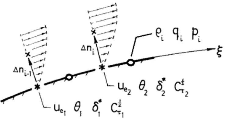
Another way to do this is to use an integral form of the boundary layer equation, such as the von Karman momentum integral used by Drela and followed in this work. As mentioned earlier, the Von Karman equation 3.43 is evident from the integration of the momentum equation 3.41a of the Thin Shear layer. Regarding the resistance estimation, the boundary layer contribution is shown in two different forms.

Another way to consider it is to integrate the shear stress along the membrane, τw.

Viscous-Inviscid Interaction

With an inverse method, not only the boundary layer is solved inversely, but also the invisible flow, which causes problems if you try to achieve this with Euler codes, for example [40]. In this method, the boundary layer is resolved via a reverse procedure, while the inviscid flow is resolved in a direct manner. Another type of approach is a quasi-simultaneous method, where a simple approximation of the inviscid flow, called Interaction Law, is solved together with the boundary layer equations, which is up-.

The first involves modifying the actual geometry of the body by adding boundary layer displacements calculated, for example, to the positions of nodes.

Implementation

4.1 2D Aerodynamic solver

4.1.1 2D Panel Method

Boundary Layer model

The delay equation 3.60 is discretized differently so as not to make it "spatially stiff" [23], giving rise to Equation 4.3. 4.3) The amplification equation used to detect transition, Equation 3.63, becomes Equation 4.4. From that position, the velocity field is separated into two, corresponding to the upper and lower surface boundary layers. The calculation continues to the following stations with the equations presented in Section 3.3.3, until the trailing edge is reached.

If transition did not occur while over the surface, transition is forced in the second coil section as laminar flow is not usually important in aerodynamic flows [23] due to the velocity flexures present at the trailing edge.

4.1.3 2D Viscous-Inviscid Interaction procedure

The results obtained show a significant error in the development of the boundary layer parameters compared to the results of the bibliography. This is justified by the fact that only one VII interaction is performed for the implemented direct code due to an anomalous behavior with the iteration number. This may be because each iteration reassembles the results into the 3D geometry and runs the Inviscid solver for this 3D geometry.

In this way, the divergent tendencies on certain sections of the boundary layer are smoothed out in the direction of the span with the adjacent sections, which makes it possible to perform more iterations and consequently significantly reduce the errors committed.

4.2 3D Aerodynamic module

Figure 4.2 shows the results obtained for a NACA 0012 airfoil at an angle of attack of 5 degrees in a flow with a Reynolds number of 106. These results are compared with those obtained using the XFOIL code [37], presented in [31] , which reflect the possible results to be obtained with a fully simultaneous approach. Cf presents a maximum error of about 60%, underestimating the actual value, and δ∗ is overestimated with a maximum error of 90%.

However, as will be seen in the following sections, when applied to a 3D Geometry, the method stabilizes.

4.2.1 3D Panel method

In this work, the GUI is used once, only when a new geometry or other discretization needs to be evaluated, at the beginning of the implementation of a wing model for the Aeroelastic framework. In this way, the boundary shear effect is taken into account when solving the inviscid problem and thus when calculating velocity and pressure distributions, as well as when calculating the resulting lift, moment and induced drag. Modifying the code to accept the inclusion of the transpiration rate would be labor intensive, so boundary layer displacement in the wake is not accounted for in the 3D VII code.

This is believed to result in an overestimation of the lift coefficient and have effects in the development of the boundary layer, i.e. the effects of the presence of the boundary layer may be underestimated.

4.2.2 3D Viscous-Inviscid interaction Procedure

Structural module

Although the method can be used in many fields, including Aerodynamics or Heat Transfer, its use in Structural Mechanics is by far the most consensual, since very good results can be obtained in structural analysis with relatively low computational requirements. With various formulations and element types available, it is the industry standard for Structural Analysis in all engineering fields. Aerodynamic pressure and shear stresses are organized and passed to the NASTRAN structural analysis file, replacing any existing load cases.

NX NASTRAN is then invoked and the results output file is generated containing, among other things, the nodal displacements.

Aeroelastic framework

Its key component is NX NASTRAN, a commercial Finite Element Analysis tool that solves the structural linear system consisting of the wing structure attached to the base and loaded with different load cases corresponding to different aerodynamic loads.

Results

Problem definition

• Wing geometry
• Flight Conditions
• Wing Aerodynamic model
• Wing Structural model

This condition was determined by taking the eClvs curve. α of the wing at the new flight speed and altitude. This was considered because under the conditions of the first test case, the high figure for the angle of attack was considered to tend to induce significant areas of separated flow. However, as can be seen in 5.4, the convergence of the aerodynamic coefficients with the number of panels used is slower for the highest angle of attack, which means that the possible presence of Boundary Layer separation along the upper wing surface it would probably require further refinement. geometry for better accuracy of the result, especially in the case of the Moment CoefficientCm.

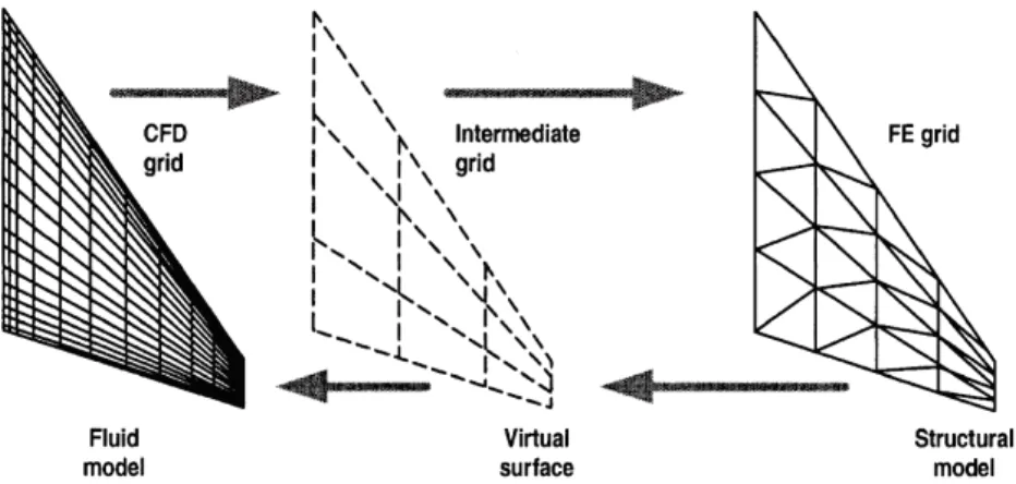
Second, as a way to simplify the implementation of the aerostructural interaction procedure, the structural mesh of the wing skin coincides with the aerodynamic and current boundary layer.

Aerodynamic Analysis Results

This was done by checking whether the Von Mises stresses in such a condition reached the yield stress of the used aluminum alloy at any position in the structure. Although these are not the only constraints or verifications to be performed when performing wing structure design, the main scope of this work focuses on the aeroelastic interaction rather than on structural design, and it was therefore considered that this type of assumption was sufficient to evaluate aeroelastic frame performance in comparative studies. a) Convergence of the lift coefficient with α= 3.5o. These results were obtained through the implementation of the geometry and flow conditions in the commercial CFD package StarCCM+.

The lift coefficient is most overestimated by the inviscid solver APAME, as expected due to the shear effect of the boundary layer not being taken into account, with an error of 8.2% for case #2.

Aeroelastic Analysis Results

• Aeroelastic Solution for Case #1
• Aeroelastic Solution for Case #2

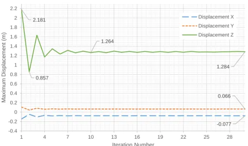
This is primarily a result of the reduction of lift due to the presence of the boundary layer. By comparing the results between inviscid and viscous assumptions, it is possible to see that the effect of the boundary layer is not negligible. For the inviscid solver, the displacements (Figure 5.15) are significantly lower than those seen for Case #1, as the lift generated was reduced in the new state.

For the Viscous case, the displacements converge faster than seen for case #1, for about 10 aerostructural iterations (Figure 5.16), with 7 VII iterations each.

Conclusions

Future Works

Starting from the aerodynamic model, more specifically the panel method, it would be very important to implement a 3D panel method code from scratch. Another reason why this would be beneficial is related to the fact that no boundary layer displacement effect could be applied to the wake geometry, as explained earlier. As for the Boundary Layer code, other 2D formulations and implementations could be tested, both simpler and more complex (as in [38]).

The sections used for the boundary layer calculation can also be obtained in different ways, such as following the flow streamlines or a combination of boundary layer flow and span calculation by separating the flow velocity into these two components.

Bibliography

Load and momentum transfer algorithms for fluid/structure interaction problems with non-matching discrete interfaces: Momentum and energy conservation, optimal discretization and application to aeroelasticity. Three-dimensional viscous flow calculations using the integral boundary layer equations simultaneously coupled with a low-order panel method. Application of a viscous-inviscid interaction panel method to determine the aerodynamic characteristics of cesar's baseline aircraft. Transactions from the Department of Aviation.

A new transformation and integration scheme for the compressible boundary layer equations and the behavior of the separation solution.