EEG correlates of fMRI dynamic functional connectivity states

Lunch breaks were essential in this job and I will forever be grateful for the gentle embrace of the civilian canteen. The internal organization of the brain can be assessed by assessing functional connectivity (FC) between brain regions using functional magnetic resonance imaging (fMRI).

Motivation

Functional Magnetic Resonance Imaging

• Basic principles
• Magnetic Resonance Imaging principles
• The BOLD signal
• Functional Connectivity in Resting-state fMRI
• Dynamic Functional Connectivity
• Dynamic Functional Connectivity States

Independent Component Analysis (ICA) is one of the most commonly used methods to identify features. The use of a sliding window is not limited to the calculation of the Pearson correlation coefficient.

Electroencephalography

Electroencephalography basic principles

• EEG frequency bands

An important parameter that must be defined a priori and that has a lot of influence on the results is the number of dFC states. They are mainly associated with deep sleep, but can also occur during the waking state [53].

EEG-fMRI

Simultaneous recording with fMRI

• Data acquisition artifacts

The GA is caused by changes in the magnetic field in the scanner due to the application of time-varying magnetic field gradients [62]. One of the most commonly used methods to correct this artifact follows an Average Artifact Subtraction (AAS) approach called image artifact reduction (IAR). Due to the roughly periodic nature of the artifact, the AAS can be used to remove it.

While turning off the lights does not present any disadvantage, in the case of the ventilation system it can cause discomfort to the patient.

State-of-the-Art

EEG correlates of fMRI dynamic functional connectivity

Inverse relationships with the alpha power were found between the anterior DMN and the medial temporal and frontal eye fields of the DAN, the parahippocampal/fusiform and superior occipital regions of the DMN and between the thalamus and the anterior DMN. To the best of our knowledge, the only study to investigate this relationship was conducted by Allen and colleagues [8], where they used an EEG-fMRI dataset acquired during eyes-open and eyes-closed conditions and EEG spectral signatures that associated with the dFCstate, try to identify. In condition 3, the visual components are less correlated with cognitive control (CC) networks and more related to the DMN, and have more occurrences during eyes closed, although with a moderate presence during eyes open;.

In A the functional connectivity matrices of the FNC states are shown, and in B their occurrence as a function of time.

Objectives and Thesis Outline

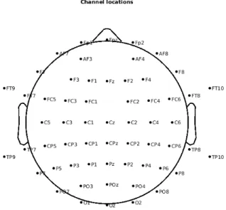
The functional data were acquired using a 2D simultaneous multi-slice gradient-echo Echo-planar imaging (EPI) sequence with aTR = 1 s and a 2.2 mm isotropic resolution. Regarding EEG data, it was acquired using two 32-channel BrainAmp MR Plus amplifiers (Brain Products, Munich, Germany) combined with a BrainCap MR model (EasyCap, Herrsching, Germany). The cap with 64 electrodes was arranged in an extended 10-20 system, with a reference on channel FCz and an electrode used to record the electrocardiogram (ECG) signal, located on the back of the subject.

All participants (or their legal representatives) gave written informed consent and the study was approved by the Lausanne ethics committee.

Pre-processing

Then, each participant's T1-weighted structural image was segmented in the GM tool, WMand CSFusing Advanced Normalization Tools (ANT) Atropos [ 74 ], to obtain an aWMandCSF mask. Functional images were then co-registered to each subject's structural space using FSL's FMRIB Linear Image Registration Tool (FLIRT) tool, and a subsequent co-registration was performed with the Montreal Neurological Institute (MNI) template using the FSL's FMRIB Nonlinear Image Registration Tool (FNIRT)) [72,75]. These ROIs were then co-registered to the patient's functional space, and the preprocessed BOLD data were averaged within each ROI.

The following steps were performed for this dissertation using MATLAB R2016b (The Math-Works Inc., Natick, MA, USA).

Dynamic Functional Connectivity Estimation

• Sliding-window Pearson Correlation
• Phase Coherence
• Comparison of dFC matrices

As for the Hilbert approach, the first step was to apply a second-order Butterworth bandpass filter in the Hz range, the same filter used in the Pearson sliding window correlation approach. However, since our goal is to compare the instantaneous phase obtained using complex Morlet wavelets and the Hilbert transform, the approach was to use the Morlet wavelets to create a band-pass filter in the same interval as that used in the Hilbert approach. Only the dFC matrices obtained by the Hilbert approach were compared with the sliding window Pearson correlation dFC matrices, as the BOLD signal was passed in the same frequency range (Hz), using the same filter only in these two approaches .

Therefore, the average of the dFC matrices obtained by the PC method was calculated in a window of the same length and time step used in the sliding window approach (35 and 5 TRs, respectively).

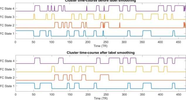
Because the algorithm can get stuck in local minima to avoid the algorithm was run 1000 times and the best result (the one where the distance of each cluster point to its center was minimum) was chosen. The k-means algorithm returns the number of k centroids as well as the label assigned to each leading eigenvector given as input to the algorithm. The clustering of each leading eigenvector takes into account only the distance between the leading eigenvector and the center of the cluster and has no time factor, so sudden changes of dFC states (labels) from one time instant to another are not allowed.

One way to tackle this problem is to apply a temporal smoothing to the labels so that each leading eigenvector is assigned not only to a cluster centroid based on its distance to it, but also the labels of the nearest leading eigenvectors Take into account.

EEG Data Analysis

Pre-processing

A major problem with the k-means algorithm is that the number of clusters must be given a priori, even if it is not known. The k-means algorithm was run with a number of clusters from 3 to 15, using the squared Euclidean distance as the distance metric for minimization. The chosen value for λ was 0.5 and the window size was chosen according to the highest frequency present in the BOLD signal, i.e. if the highest frequency is 0.1 Hz then the window would have a size of s.

Spectral analysis

The average power in the mentioned bands was obtained by dividing the entire band analyzed (1-20 Hz) into four frequency bands: delta [1,4]. Note that the beta band usually goes up to 30 Hz [54,55], but due to the reason above, the frequency limit is 20 Hz.

EEG-fMRI analysis

EEG correlates of dFC states

• Taking into account the haemodynamic response function

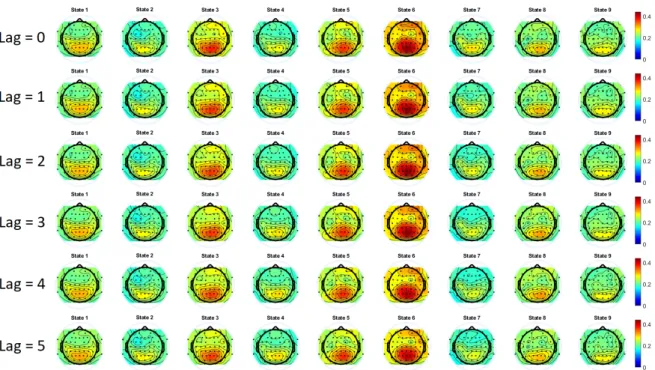
To investigate whether, taking into account the delay between the EEG spectrometrics and the fMRI dFC states introduced by the hemodynamic response function would affect the previously obtained results, a delay was introduced into the EEG-fMRI data in the range of 1 to 5 s, corresponding to realistic values ​​of the hemodynamic delay. Since fMRI data is the one that is delayed, the higher the delay, the more initial samples of each subject were omitted. For the EEG data, the omitted samples were the last of each subject.

The introduction of the delay was done exclusively for the results passed in 0.01-0.1 Hz in a band.

Characterization of dFC states

Comparison between Phase Coherence dFC matrices obtained using Hilbert transform

In Figure 3.1, the distribution of the cosine similarity calculated between the dFC matrices obtained with PC and Pearson correlation with the sliding window is illustrated for all 9 subjects (top) and for each subject individually (bottom). The cosine similarity values ​​obtained for all subjects are above 0.56 and moreover 99.996% of the values ​​are between 0.73 and 0.99 (all data points except the outliers). On the left, the boxplot represents the distribution of the cosine similarity values ​​for all subjects.

The distribution of cosine similarity calculated between dFC matrices obtained by PC using the Hilbert transform and Wavelet transform methods is shown in Figure 3.2.

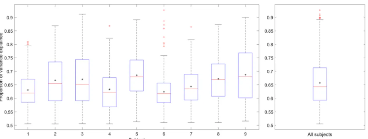
Leading eigenvector explained variance

Thus, at the beginning and end of the BOLD signal, there is no signal information before and after, respectively, which means that at these time points the signal resulting from the convolution may not be well estimated. However, since this is a comparison analysis between two methods, the results can only warn for the estimation of dFC matrices using phase synchronization at the beginning and end of the time courses, but the conclusion to which method is better or if the first and last FC matrices are not well estimated and should be removed is not clear and further studies should take this into account. The choice of the Hilbert transform instead of the Wavelet transform rests solely on the fact that the Hilbert transform is applied to a bandpass filtered signal, so it is appropriate to analyze frequency bands of a signal, which is the case of this analysis is.

The wavelet transform, due to its Gaussian form in the frequency domain, seems more suitable when a specific frequency and its neighboring frequencies are intended to be studied, requiring some adaptations when the analysis lies in a band of the signal.

EEG spectral analysis

This difference is more pronounced in relative alpha power, where power at all time points is relatively greater than in the remaining subjects. One possible explanation could be the inter-individual variability of strength in these bands, i.e. some subjects naturally have more power than others, especially in the alpha band [84]. For any of these reasons, these results require a more detailed analysis in the following results related to the EEG bands.

On the one hand, this is good, as the results are not affected by inter-individual variability, but on the other hand, by imposing that all subjects must have their ASI between 0 and 1, it may give more importance to some values, which in fact should be lower.

Analysis on the frequency band 0.01-0.1 Hz

EEG correlates of dFC states

In the case of the ASI measurement, the number of states with the most different state topography is 4. There is also one more dFC state associated with high alpha power, which only appears at 7 states, but is retained until the highest number analyzed states. Then the maximum value was taken to select states that have higher alpha than others from different number of states.

The comparison between the maximum values ​​obtained for each number of states (3 to 15) is shown in Figure 3.10.

Characterization of dFC states

At the top is the network in cortical space, where the centroid vector values ​​are used to scale the color of each brain area, and connections (blue connections) are drawn between brain areas with a value <−0.1, highlighting the network. in contrast to the global mode. In the middle is shown the dFC matrix obtained by calculating the outer product of the centroid vector. In the lower part, the elements of each central vector and the corresponding brain regions are represented.

The top left corner shows fractional occupancy, calculated as the number of TRs each state was active over the total number of TRs.

Effect of haemodynamic response function

State 1, which is the state where there is a global coherence of BOLD phases, has the highest fractional occupancy (0.32) and the longest mean lifetime (17.8±1.8 TRs). These results indicate that after spending some time misaligned with the global signal (and aligned between them), the BOLD phases realigned with the global signal most of the time, and return to a state where all phases have the same direction. Regarding the average lifetime, it is important to note that all states have an average duration of more than 10 TRs due to the temporal smoothing applied to the labels after the K-means clustering.

Although it was not a strict smoothing, but a balanced smoothing that took into account the distance of each leading eigenvector to its centroid, as well as the neighboring labels, the minimum average lifetime could have been slightly below 10TR, however with this number of conditions they were all above 10TR.

Analysis on multiple frequency bands (slow-5 to slow-2)

The first state found in the slow-5 band is very similar to the first state found previously, with a similarity of 0.99, which is the state representing the global coherence state. The color scale used in the topographies is equal to the one used in the previous analysis. This long average lifetime actually changes the results relative to those obtained in the band 0.01-0.1 Hz.

Since neither of these modes was found in the original analysis, both had small similarity values.

Limitations and Future Work

Caffo, “Evaluating dynamic bivariate correlations in resting-state fMRI: a comparative study and a new approach,” NeuroImage , vol. Ville, “Principal components of functional connectivity: A new approach to study dynamic brain connectivity during rest,” NeuroImage , vol. Ballistocardiogram artifact correction considering physiological signal preservation in concurrent EEG-fMRI,” NeuroImage , vol.

Cox, “Mapping source correlations in resting-state FMRI, with artifact detection and removal,” NeuroImage , vol.

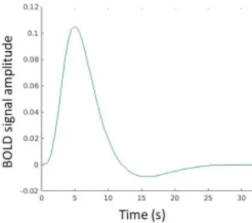
Canonical HRF

Resting state networks identified by Smith et al, 2009

Sliding-window Pearson Correlation method to extract dFC

Dynamic Functional Connectivity states obtained on Allen et al., 2017

EEG spectra averaged over all epochs and subjects, segregated by dFC states

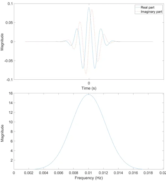
Complex Morlet Wavelet in time and frequency domain

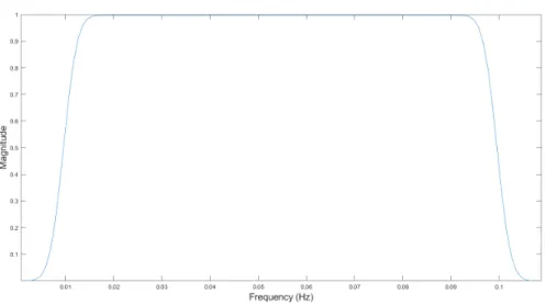
Band-pass filter created by averaging 100 complex Morlet wavelets with their Gaussian

Cluster time course for the k-means algorithm with 4 centroids

EEG channels location

Comparison between dFC matrices obtained with Phase Coherence (PC) and Sliding-

Comparison between dFC matrices obtained with the Phase Coherence method using

Cosine similarity time-course between dFC matrices obtained with the Phase Coherence

Evolution of relative power in delta, theta, alpha and beta bands over time and subjects,

Evolution of ASI over time and subjects, for all channels (different colors)

Maximum Euclidean distance between most similar state topographies for each number

Cortical representation of the dFC state and associate mean topography of relative alpha