Fast Segmentation of the Left Ventricle in Cardiac MRI Using Dynamic Programming
Carlos Santiago Jacinto C. Nascimento Jorge S. Marques
Institute for Systems and Robotics (ISR/IST), LARSyS, Instituto Superior T´ecnico,
Universidade Lisboa, Portugal
Abstract
Background and Objective: The segmentation of the left ventricle (LV) in cardiac magnetic resonance imaging is a necessary step for the analysis and diagnosis of cardiac function. In most clinical setups, this step is still manually performed by cardiologists, which is time-consuming and laborious. This paper proposes a fast system for the segmentation of the LV that significantly reduces human intervention.
Methods: A dynamic programming approach is used to obtain the border of the LV. Using very simple assumptions about the expected shape and location of the segmentation, this system is able to deal with many of the challenges associated with this problem. The system was evaluated on two public datasets: one with 33 patients, comprising a total of 660 magnetic resonance volumes and another with 45 patients, comprising a total of 90 volumes. Quantitative evaluation of the segmentation accuracy and computational complexity was performed.
Results: The proposed system is able to segment a whole volume in 1.5 seconds and achieves an average Dice similarity coefficient of 86.0% and an average perpendicular distance of 2.4 mm, which compares favorably with other state-of-the-art methods.
Conclusions: A system for the segmentation of the left ventricle in cardiac mag- netic resonance imaging is proposed. It is a fast framework that significantly reduces the amount of time and work required of cardiologists.
Key words: Cardiac MRI, left ventricle, segmentation, dynamic programming
Email addresses: carlos.santiago@ist.utl.pt (Carlos Santiago),
jan@isr.ist.utl.pt(Jacinto C. Nascimento),jsm@isr.ist.utl.pt(Jorge S.
Marques).
1 Introduction
The diagnosis of cardiomyopathies is recognized primarily as a fundamental requirement for the patient throughput. A crucial step in the analysis of car- diac function is the identification of the endocardium, the inner border of the left ventricle (LV). With this information, important medical features can be determined, namely, the left ventricular volume and the ejection fraction, which are amongst the most used parameters in the diagnosis and prognosis of heart diseases.
Quantitative assessment raises as a natural stage towards the diagnosis, in which magnetic resonance imaging (MRI) is considered the gold standard in the assessment of left ventricular function as a non-invasive image modality.
However, to accomplish such quantitative assessment in MRI, an accurate segmentation of the LV is mandatory.
In the majority of the clinical setups, the segmentation of a magnetic resonance (MR) volume is manually performed by cardiologists, in a time consuming and demanding process. A typical magnetic resonance (MR) volume comprises 8 to 15 slices, and requires roughly 13 to 17 landmark points to delineate the LV contour. Furthermore, this manual intervention is required in theend-diastolic and end-systolic phases of the cardiac cycle [1], which means a total of more than 200 points have to be manually introduced by cardiologists in order to proceed with the diagnosis. This means that a (semi)automatic segmentation method that reduces the amount of work required is highly desirable.
In this paper, we address this problem using a fast dynamic programming (DP) methodology inspired in [2,3]. This approach is based on two main assumptions about the LV border: 1) that it is approximately circular in each MR slice;
and 2) that it is (at least partially) associated to edges in the image. The segmentation of each MR slice is performed in polar coordinates and involves the following steps. First, an edge map is built so that its valleys roughly correspond to location of the LV border. Second, a Dynamic Programming algorithm is applied to determine the optimal path along the edge map, which corresponds to the delineation of the LV contour.
The paper is organized as follows. Section 2 describes related work in the field. Section 3 details the methodology and the contributions herein proposed.
Section 4 describes the experimental setup and a comparative study with state- of-the-art related approaches is performed. Concluding remarks are addressed in Section 6.
2 Related Work
Although there are several methods dedicated to the MRI segmentation, the problem is still open, motivating not only several surveys available in the liter- ature [4,5], but also several challenges,e.g., MICCAI 2009 and 2011, resulting in a LV segmentation challenge consensus paper [6]. In fact, the automatic endocardial delineation is a task that is far from being straightforwardly ac- complished. In the following, we describe the challenges of this task and how they have been tackled in the related literature.
2.1 Challenges in the MRI Segmentation of the LV endocardium
One of the main challenges associated with this problem is the fact that some parts of the LV border may not always be associated with image edges. This caused by the presence of the gray level inhomogeneities, due to the blood flow, and by the presence of papillary muscles and trabeculations, or wall irregularities, inside the heart chambers, that have the same intensity profile as the endocardium. As such, some image features such as intensity and gradient do not represent the real contours near the papillary muscle. Motivated by the fact that clinicians consider the papillary muscle trabeculations within the LV cavity [1], this could be a source of inaccuracies in automatic segmentation algorithms. Several works have been published to tackle this issue, e.g., by computing the convex hull of the contour [7,8] or by adopting morphological operations [9,10].
The segmentation of the apical and basal slices also faces additional challenges [11]. The apical slices are difficult to segment because the MRI resolution is too coarse to provide detailed and good visualization of small structures at the apex. Regarding the basal slice, there exists large LV shape changes near the base of the heart due to its vicinity to the atria.
Other issues include: unpredictable end of the LV cavity, vicinity of the di- aphragm, large shape variability, and tissue motion and haziness [4].
2.2 Image based methodologies
As mentioned above, the presence of papillary muscles, as well as the trabec- ulations provide gray level inhomogeneities in the endocardium contour. To tackle this challenge several works have been published in the attempt to seg- ment the endocardium of the LV. One class of approaches is based on a thresh- old operation [12] to separate outer and inner regions of the contour. However,
DP is one of the most common choices for data-driven endocardial/epicardial border detection. This class of approaches is rooted in the work of Geiger et al.
[13] and used in several works,e.g.[2,7,14–17]. It searches for the optimal path (i.e., the contour) by using a cost matrix that assigns a low cost to the object boundary. The design of the cost matrix itself is a challenging task and plays a core role in DP based approaches, which motivated research on this subject.
In [7], a threshold based approach is presented, in which the optimal threshold is found by computing the mean gray value of the maximal edge pixels. These pixels are found by generating orthogonal lines radiating from the epicardial center and collecting, for each line, the gray intensity of the pixel with highest edge value (i.e., maximal edge) within the epicardial contour. A methodology termediterative multigrid dynamic programming (IMDP) is introduced in [2].
Here, the contours of the LV in ultrasound image sequences are assumed to be one dimensional noncausal first order Markov random fields. The DP is run in a multigrid fashion, i.e., first with a coarse resolution, followed by a refining stage that estimates the segmentation by searching in a smaller range, using a thinner resolution. To obtain the cost matrix, they model the inten- sity values of the tissues surrounding the ventricle border. DP has also been used to extract the myocardium region in [17]. First, they identify the endo- cardium border by using a classifier to label the LV cavity pixels and applying a convex hull operation on that region. Then, the image is converted to polar coordinates and transformed into a cost matrix based on the gradient along the radial direction. Finally, DP is applied to determine the epicardial border.
In order to obtain a closed contour, they iteratively extend the cost matrix by replicating the initial part until they find an end point that intersects with the contour.
In [18] a threshold based operation is also used, where the binary masks (i.e., thresholded images) are jointly used with the Global Circular Shortest Path algorithm (GCSP). It is shown that an improved method is achieved by com- bining the advantages of the two above techniques together. Fuzzy logic is used in [14] that comprises two stages. The first stage accounts for the pixel gray values and presence of edges, while the second stage comprises the deter- mination of cardiac contours that is based on fuzzy logic with DP. With these two ingredients, a degree to which each pixel belongs to the cardiac contour is computed, allowing the image to be represented by a membership degree matrix. The final step comprises a graph search on the cost matrix to deter- mine the cardiac contour. In [15] histogram equalization followed by wavelet transform is used to build the cost matrix. The branch-and-bound algorithm is used [16], where the main focus is to reduce the complexity of finding the optimal path that represents the endocardial border. In [10], the endocardial border is obtained for each volume independently using a region growing tech- nique called geodesic dilations [19]. The idea is to merge two regions inside the LV cavity: one located close to the LV center that has a higher intensity, and another one located closer to the border, whose intensity is lower due
to the proximity to the muscle tissue. A shortest path algorithm is also used in [20], which averages all the phases over one cardiac cycle, and contours in each image can be recovered using minimum surface segmentation. Spectral decomposition is another image based approach that has been used to seg- ment the LV in [21]. It allows them to represent the images independently of the imaging modality and specifications, from which they employ a clustering step that divides the images into superpixels of similar appearance and their corresponding labels.
2.3 Deformable models
Another class of approaches regarding object segmentation is the active con- tours (or deformable models). The seminal approach is rooted in [22], which consists of an optimization problem that moves a parameterized curve toward image regions with strong edge information. Related approaches concerning this trend are characterized by a geometric representation that covers a large variability of shapes, and is currently used in medical image segmentation (e.g., [23,24]).
The deformable model designation stems from the use of elasticity theory within a Lagrangian dynamics setting. The above setting, is characterized by forces that are internal to the model, which are calledinternal forces (related to the prior), and the external potential energy functions that are defined in terms of data of interest in the image (e.g., boundary of the object to be segmented). These potential energies are associated to the external forces that are able to deform the model to fit the desired data. The energy of the deformable model is supposed to be minimal when two conditions are reached:
(i) the model is located at the desired boundary (low external energy) and (ii) has a shape which is supposed to be relevant considering the shape of the object being sought (low internal energy).
The deformable models have been largely used, due to its success at segment- ing the LV. Since the success of the gradient vector flow (GVF) applied in snakes [25], this has motivated the use of deformable model based approaches to segment the LV in MRI. In [26], the GVF is used for segmenting the heart in MRI, however disregarding the consequences of the papillary muscles and ar- tifacts. Variations of the GVF have also been proposed, such as in [24], where Hough transform is applied to intensity difference image to locate the LV cen- troid with a new external force termed asgradient vector convolution (GVC).
In [27], an Iterative Thresholding and an Active Contour model with Adap- tation (ITHACA) were presented to segment the endocardium. In [28] several external forces were studied as extensions of the snake to assess the distance between computer-generated and the observer’s hand-outlined boundaries, to
perform a systematic comparison. The main outcome is that, although there is an agreement between manual and segmentation algorithms for ejection frac- tion, the end-systolic and end-diastolic volumes are underestimated. Level-set approaches have also been used to retrieve the endocardial border. For in- stance, in [29], an energy function based on edge information is used with two combined level-set models to obtain the endocardial and epicardial borders.
The introduction of prior models of the LV in the snake has also been explored.
Several alternatives for the LV prior have been explored in the literature, for instance using elliptic shape prior [30], intensity based priors [31], which pre- vent the papillary muscles from being included into the heart myocardium. In [32] a statistical classifier is introduced, trained using feature selection that allows an appropriate weighting of the most relevant features. Also, large train- ing sets have been used to build the LV shape statistics prior. This has been applied not only in MRI [32,33], but also in other image modalities, such as in the ultrasound [34,35]. More recently, Avendi et al. [36] proposed a deep learning approach to locate the LV in the image and compute a shape prior, which is used to constrain a deformable model to improve its accuracy.
2.4 Contributions
In this work, we follow the algorithm proposed in [3] for crater delineation.
This approach relies on DP to extract the desired boundary by analyzing the image in polar coordinates. This approach is distinct from other methods in the literature in the computation of the cost matrix for the DP algorithm, which is based on a normalized edge map. We propose to combine this analy- sis with the enhancements to the DP algorithm proposed in [2], which allows significant improvements in terms of computational complexity, without com- promising the accuracy of the segmentation. This means that the algorithm is able to determine the location of the LV border very quickly and provides accurate medical parameters (namely, the ejection fraction). Furthermore, this approach guarantees that the optimal path provided by DP is a closed con- tour, without the need to enlarge the edge map, as in [17], which also helps improve the efficiency of the algorithm. Finally, we include an additional step that is specific for cardiac MRI segmentation, which consists in automatically updating the information about the center and radius of the expected segmen- tation. This allows the algorithm to accurately segment the whole MR volume without the need for additional user input.
Section 3.1
Section 3.3 Section 3.2
Inputs
Transform to polar coordinates
Determine contour with DP Segmentation
Compute edge map
Update c and R estimates Stopping
criteria Select image
ROI Initial guess of
c and R
y
n
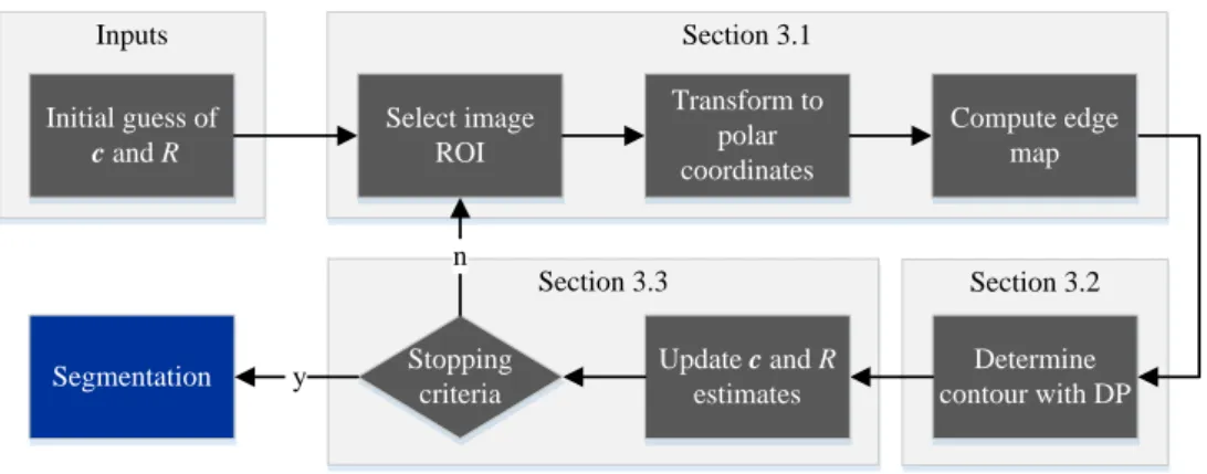
Fig. 1. Overview of the proposed methodology applied to each slice of the MR volume, where c and R denote the coordinates of the center and radius of the LV, respectively.
3 Proposed Methodology
The goal of the proposed method is to provide a fast and accurate segmen- tation of the LV in MR volumes. We address this problem by sequentially analyzing the slices (2D images) in a given volume. Starting with an initial guess of the location of the LV in the basal slice, the proposed algorithm aims to determine the location of the endocardium in that particular slice. This initial guess is obtained by user input, although this step could be replaced by an automatic method, such as using the Hough transform for circles, or using the approach proposed in [20]. This segmentation is then propagated to the next slice as an initial guess, and the algorithm is applied to this new slice. This procedure is repeated until all the slices in the volume have been segmented.
Fig. 1 provides an overview of the proposed approach, illustrating the main steps that are performed for a given slice of the MR volume. The methodol- ogy herein proposed is based on the following two main stages: (i) conversion of the original image (MR slice) into an (inverted) edge map, whose valleys are considered as coarse candidate positions for the endocardium; (ii) com- putation of the optimal path along the edge map, which corresponds to afine estimation of the location of the endocardium.
Concerning the first stage, we follow the approach proposed in [3]. Based on an initial guess of the LV center and radius, this algorithm converts the MR image to polar coordinates. Then, a gradient operator is applied along the radial dimension, in order to extract possible candidates for the location of the LV border. Finally, the resulting gradient image is transformed into an edge map that penalizes pixels with low gradient.
Typically, edge detection is not a reliable approach in this image modality
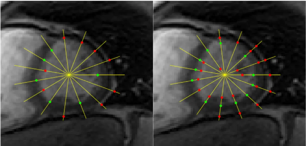
Fig. 2. Detection of edge points (bright to dark) along the yellow lines. On the left, only the strongest edge point in each line is shown, and on the right all the detected edge points are shown. Green dots belong to the LV border and red dots are outliers.
(recall Section 2.1). An example is illustrated in Fig. 2: in the left image, the edge points with higher gradient along the yellow lines are shown; in the right image, all the edge points (local gradient maxima along the yellow lines) are shown. The edge points in red are outliers whereas the green ones belong to the endocardium. In both cases, it is possible to see that many edge points are outliers, and that LV border is not always located along image edges.
Therefore, additional information is required to avoid being misguided by these outliers.
The goal of the latter stage is precisely to extract a curve that satisfies specific shape constraints while still being able to follow the valleys of the edge map (i.e., avoid going through pixels with low gradient). This trade-off between the constraints and the image information allows the algorithm to avoid erro- neous edges related to papillary muscles and other misleading structures. The optimal curve is then converted to Cartesian coordinates for the segmentation of the LV to be obtained.
Once these two stages are complete, the LV center and radius can be recom- puted from the segmentation. The updated parameters are used to determine if the initial guess was in agreement with the segmentation or if a new iter- ation is required. This iterative process allows the algorithm to recover from poor initial guesses.
The two stages of the proposed approach are analytically described in Sections 3.1 and 3.2, respectively. The update of the LV center and radius in described in 3.3.
3.1 Computation of the edge map
In this stage, the goal is to compute an edge map from the original MR image, such that its valleys follow the LV border (see top right box in Fig. 1). Since the morphology of the LV is roughly circular, this step is performed in polar coordinates, as in [2].
In order to obtain a representation of the MR image in polar coordinates, an initial guess of the LV’s center, denoted by c = [cx, cy]> ∈ R2, and its size, R∈R, have to be provided. Then, the intensity of a particular pixel (r, θ) in the image in polar coordinates is obtained by computing
IP(r, θ) =I(x, y), (1)
where the pixel position correspondence is given by
x=cx+rcos(θ), y=cy+rsin(θ). (2) This transformation does not guarantee thatx, ytake integer values, thus we use bilinear interpolation to obtain the value of IP(r, θ) (see [37]). The pairs (r, θ) for whichIP is defined belong to the domainDr× Dθ,
Dr =nr1, . . . , rM ∈R:ri =rmin+ (i−1)∆r, i= 1, . . . , Mo (3) Dθ =nθ1, . . . , θN ∈[0,2π] :θj = (j−1)∆θ, j= 1, . . . , No, (4) where ∆r = rmaxM−r−1min, and ∆θ = N2π−1. The maximum and minimum radii, rmax andrmin, define the width of the ring within which we expect to find the LV border. Also note that θN = 2π =θ1, i.e., the pixels in the left and right borders of IP correspond to the same positions in the original image.
OnceIP(r, θ) is computed, a high-pass filter,H, is applied to obtain the radial gradient imageIG(r, θ). We are only interested in computing the gradient along r, and in transitions from bright to dark, as those depicted in Fig. 2. The impulse response of the high pass filter is given by
H(r) =
1 if 0< r≤T
−1 if −T < r≤0 0 otherwise,
(5)
where T is a user defined parameter (in the results section, this parameter was set to T = 6). The radial gradient image is obtained by applying the convolution operator
IG(r, θ) =IP(r, θ)? H(r). (6) Notice thatIG(r, θ) takes values in ]−∞,∞[, in which: 1) large, positive values correspond to edges such as the ones associated with the LV border; 2) large,
(a) (b) (c) (d)
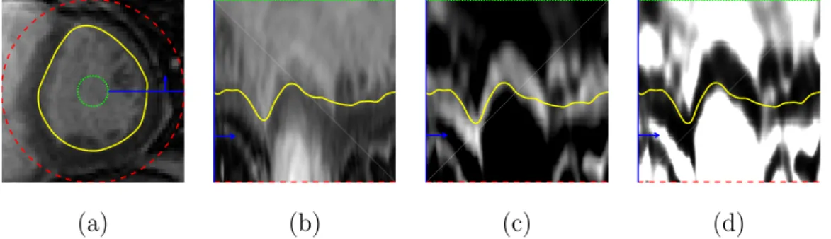
Fig. 3. (a) Original LV image, I(x, y); (b) image in polar coordinates, IP(r, θ); (c) image gradient,IG(r, θ); and (d) edge map, eMAP(r, θ). The yellow line corresponds to the LV segmentation. The green and red lines correspond to the minimum and maximum radius, respectively, and the blue line and arrow help illustrate the con- version to polar coordinates.
negative values correspond to edges with the opposite gradient direction (from dark to bright); and 3) values close to zero indicate the absence of edges.
We wish to transform IG(r, θ) into a cost map, such that the desired edges have zero cost and every other possibility has a cost of approximately 1. To accomplish this, the sigmoid function proposed in [3] is adopted:
eMAP(r, θ) = 1
1 + expλ(IG(r, θ)−k), (7) wherek > 0 controls the inflection point, andλ >0 controls the sharpness of the sigmoid. In this work, good values for these parameters were empirically determined to be k = 20 and λ= 0.04.
The edge map, eMAP(r, θ) ∈ [0,1] is now normalized, and its valleys corre- spond to rough candidate positions of the LV border. Fig. 3 illustrates the whole pre-processing stage, from the original MR image, I(x, y), in Cartesian coordinates, depicted in Fig. 3 (a), to the final edge map, eMAP(r, θ), in polar coordinates, depicted in Fig. 3 (d), whose valleys follow the path of the LV border, shown in yellow.
3.2 Contour estimation
The second stage of the algorithm aims to perform the delineation of the LV boundary (bottom right box in Fig. 1), computed from the output of the previous stage. More specifically, the goal is to find a curve that follows the valleys of the edge map, eMAP (e.g., the yellow line depicted in Fig. 3 (d)).
In the original Cartesian coordinates, a popular approach to address this prob- lem is the following: find a parametric curve, x(s) = (x(s), y(s)), which is ab
function of the curve parameter, 0≤s≤1, such that xb = arg min
x E(x), (8)
where E is a cost function analytically defined as E(x) =
Z
s
Eint(x(s)) +Eext(x(s))ds. (9) The first term in (9) is an internal energy (i.e., the prior), typically imposing a smoothness constraint. The second term corresponds to the external potential energy function that is defined in terms of the image data, e.g., the edge map eMAP defined in Sec. 3.1. This approach is commonly used in the deformable contours literature [38,39].
In this paper, we wish to address a similar problem but in discrete polar coordinates. Recalling that the edge map, eMAP, can be viewed as a M × N matrix, the goal is to determine the curve br = [r(1), . . . , r(N)]> (i.e., a sequence of radius values), such that r(j)∈ Dr corresponds to the LV radius for angle θj (recall (3) and (4)). Similarly to (8), the curve br is obtained by computing
br= arg minr E(r)
s.t. r(1) =r(N)
r(j)∈ Dr, j = 1, . . . , N
(10)
The constraint r(1) = r(N) is required to guarantee that br is a closed curve in Cartesian coordinates. In this case, the cost function E(r) is defined as
E(r) =
N
X
j=1
Eint(r(j)) +Eext(r(j)), (11) where the image-related term is given by
Eext(r(j)) = eMAP(r(j), θj), (12) and the prior term,
Eint(r(j)) =d(r(j−1), r(j)) (13)
=
0 if |r(j)−r(j−1)|= 0 η if |r(j)−r(j−1)|= ∆r
∞ otherwise
. (14)
is used to impose a smoothness constraint on curve r, by penalizing large variations in consecutive pairs (r(j−1), r(j)), withEint(r(1)) = 0.
By replacing (12), (14) into (11), the global cost function can be rewritten as E(r) = eMAP(r(1), θ1) +
N
X
j=2
eMAP(r(j), θj) +d(r(j−1), r(j)). (15)
Note that this cost function is a sum of local cost functions. Therefore, the optimal cost can be recursively computed through DP [40].
LetEj(ri) denote the optimal cost of reaching a specific position, (ri, θj), in the image, starting in the first column (θ1). This cost can be recursively computed using the optimal costs for reaching the positions in the previous column
Ej(ri) = eMAP(ri, θj)+ min
ρ∈Dr
d(ρ, ri) +Ej−1(ρ)
. (16)
However, there is a global constraint, expressed in (10), which demands that r(1) = r(N). In order to satisfy this constraint, the problem defined in (10) can be subdivided into M subproblems: for each subproblem, we choose a different initial value for r(1) ∈ Dr, and impose that the optimal path starts in this position. This is achieved by changing the first column of the edge map to eMAP(ri, θ1) =∞,∀ri 6=r(1), i= 1, . . . , M (all the paths that do not begin inr(1) will have infinite cost). Then, the following two steps are performed:
(1) Forward step: Compute the optimal costs of all the curves that start at θ1 and end at θN, using (16), and, for each local minimization problem (second term in (16)), store the corresponding radii
φ(ri, θj) = arg min
ρ∈Dr
d(ρ, ri) +Ej−1(ρ). (17) (2) Backward step: Trace back the optimal path that ends at r(N) = r(1),
by using the radii stored in the previous step
r(N) =r(1) (18)
r(τ −1) =φ(r(τ), θτ), τ =N, ...,2 (19) The Algorithm 1 summarizes the process of applying DP to find a candidate LV contour starting at a specific position, r(1).
This process is repeated for all possible starting point r(1) ∈ Dr. Then, the path with the lowest global cost (computed using (15)) is selected as the proposed segmentation.
Notice that running Algorithm 1 (A1) for all starting positions may be costly, depending on the number of possibilities,M. Alternatively, Bioucas-Dias et al.
[2] proposed to alleviate this by only running A1 two times (2-loop algorithm).
They assume that the optimal path close to j = N/2 is not influenced by the initialization, r(1). Thus, for whatever starting position they choose in
Algorithm 1Determining the best LV contour candidate starting at r(1) for all ri 6=r(1) do
E1(ri) = ∞ end for forward step for j = 1 to N do
for i= 1 to M do
compute Ej(ri) using (16) compute φ(ri, θj) using (17) end for
end for backward step
select ending point r(N) =r(1) for j =N to 2 do
r(j−1) = φ(r(j), θj) end for
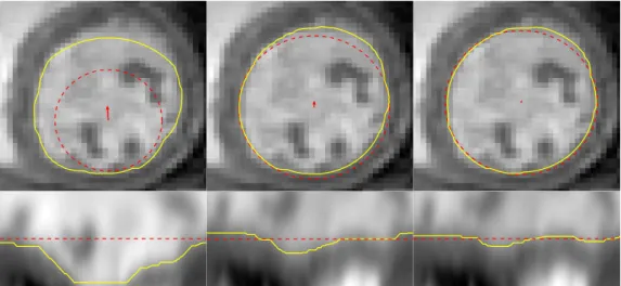
Fig. 4. 2-loop algorithm [2]. The blue line depicts the solution of A1 with initial position r(1) = rmin; the red line depicts the solution of A1 on the reordered edge map with initial positionr0(1) =r(N/2); the green dashed line represents the ground truth segmentation. The yellow and magenta rectangles and black arrows illustrate how the reordering of the edge map and the optimal path works.
the first run, say r(1) = rmin (blue curve in Fig. 4), the optimal value for r(N/2) will always be the same. Under this assumption, they simply reorder the two halves of the edge map, as illustrated by the colored rectangles in Fig. 4 (center), and run A1 a second time, starting at positionr0(1) =r(N/2), wherer0 = [r0(1), . . . , r0(N)]>denotes the optimal path on the new (reordered) edge map. To obtain the solution for the original edge map, the two halves of r0 are rearranged back to the original order (red curve in Fig. 4 (right)). This way, the complexity of the algorithm is reduced, allowing the segmentations to be obtained significantly faster and independently of the choice of M. Once the optimal (or sub-optimal) path has been computed, the LV segmen- tation in the original Cartesian coordinates, denoted by x, is obtained by
transforming the coordinates of each point in r as follows
x(j) =c+r(j)hcosθj,sinθji>, j = 1, . . . , N. (20)
3.3 Automatic estimation of the cand r parameters
The algorithm described above provides a path r ∈RN that defines the con- tour of the LV along the edge map, eMAP. However, this path provides a good estimate of the LV border under the premise that the LV is roughly a circle with a specific center, c, and radius, R ∈ Dr (recall (2) and (3)). In most cases, these parameters are provided by using the segmentation obtained in the previous slice, which may be inaccurate. Consequently, the resulting LV segmentations may not be correct. This section describes how the estimates of R and c are refined based on the “optimal” path r (see Fig.1).
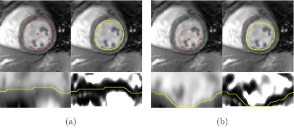
The initial premise that the LV is roughly a circle on the MRI slice means that the path r is expected to be roughly a horizontal line along the edge map, eMAP. Moreover, if the initial estimate of the LV radius, r, is accurate, then the straight line should be located along the middle of the edge map, as shown in Fig. 5 (a). An example of the segmentation obtained from inaccurate estimates of R and c is depicted in Fig. 5 (b). On one hand, an inaccurate estimate of the centercleads to a sinusoidal curve along the edge map, instead of a straight line. On the other hand, an expected radius smaller (larger) than the actual LV radius leads to a curve that is closer to the bottom (top) part of the edge map (see Fig. 5 (b)). In the extreme case, the segmentation may not be able to follow the actual LV contour, as shown in the figure, leading to a path that follows the border of the edge map. Thus, it is necessary to update the estimates of R and c. This can be achieved through the analysis of the path, r, as follows.
Let ¯r be the average distance of the contour to the center estimatec
¯ r = 1
N
N
X
j=1
r(j), (21)
wherer(j) is thej-th component ofr. The estimate of the expected LV radius is updated by
R ←r.¯ (22)
Now, let p(j) ∈ R2 be the position of the j-th contour point, associated to
(a) (b)
Fig. 5. Examples of the segmentation obtained from (a) an accurate and (b) an inaccurate estimate of the LV radius, R, and center, c. For each case, we show the original MRI slice (top), the MRI slice in polar coordinates (bottom left), and the edge map (bottom right). The red circles are the initial estimate of the cen- ter and radius (top left and right) and the yellow curves show the corresponding segmentations obtained using the proposed algorithm.
Fig. 6. Example of the updated estimates ofc andR, and corresponding segmenta- tions. The first column shows the initial center and radius estimate and the following columns show new iterations of the update scheme. The red circles depict the center and radius estimates and the yellow curve shows the corresponding segmentation.
The red arrows correspond to the center update.
r(j) and θj, in Cartesian coordinates
p(j) = c+r(j)
cosθj
sinθj
, (23)
and letc be defined as the centroid of those points, c= 1
N
N
X
j=1
p(j). (24)
The updated estimate of the LV center is obtained by
c←c. (25)
This update scheme allows the path,r, to iteratively converge towards the LV border even when the initial estimate of its center and radius are inaccurate.
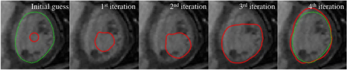
Consider the example of the inaccurate initial estimate depicted in Fig. 5 (b). Applying three iterations of the update scheme described above leads to the results shown in Fig. 6. In this figure, it is possible to see that, in each iteration, the segmentation becomes more similar to a straight line in the polar coordinates space (bottom images) and gets closer to the correct LV segmentation in the original image (top images).
4 Evaluation
4.1 Experimental Setup
The proposed method was evaluated on two public datasets of cardiac MRI sequences [11,41]. The first dataset, denoted by D1, consists of 33 sequences acquired from 33 healthy and diseased subjects [11]. Each sequence comprises 20 volumes, covering one cardiac cycle. The number of slices in each volume ranged from 5 to 10, with a spacing of 6−13 mm. Each slice is a 256×256 image, with a resolution of 0.93−1.64 mm. A ground truth (GT) of the LV segmentation in each slice is also provided. In total, dataset D1 has a total of 5011 images with the corresponding segmentations. The second dataset, denoted by D2, consists of 45 sequences, also comprising healthy and diseased subjects, that were used in the MICCAI 2009 LV segmentation challenge [41].
Each sequence has 20 volumes, over one cardiac cycle, and 6 to 12 slices, which are 256×256 images with a resolution of 1.25 to 1.56 mm. In this dataset, GT segmentations are only available for the end-diastolic and end-systolic frames. In total, dataset D2 has a total of 805 images with the corresponding segmentations.
The evaluation of the proposed algorithm was achieved using two different metrics:
(1) The volumetric Dice coefficient,dDice, which measures the percentage of
overlap between the proposed segmentation and the GT. Let S? denote a binary volume with the proposed segmentation (1’s inside the LV) and SGT be the corresponding GT. Then,
dDice= 2 V(S?∩SGT)
V(S?) +V(SGT), (26)
where V(·) counts the number of voxels with value 1, and S? ∩SGT is the intersection between the two segmentations. A segmentation with dDice = 1 is a perfect match with the GT, whereas dDice = 0 means the two segmentations do not even intersect.
(2) The average perpendicular distance, dAV, between the proposed segmen- tation and the GT, expressed in mm.
Medical parameters, namely the end-systolic and end-diastolic volumes (ESV and EDV) and the ejection fraction (EF), were also computed and compared with those obtained with the GT. Finally, we also show the results excluding
“bad” segmentations (dAV>5 mm), along with the corresponding percentage of “good” segmentations, following the evaluation strategy used in the MIC- CAI 2009 LV segmentation challenge [41]. In both datasets, the evaluation was obtained using a custom Matlab code, and not the code available for the MICCAI 2009 challenge.
In the following section, we demonstrate results using: 1) the algorithm A1 without the automatic update of c and R described in Section 3.3, 2) A1 with automatic updates (A1+AU), and 3) the 2-loop (2L) algorithm with automatic updates (2L+AU).
4.2 Results
The evaluation of the proposed method is divided into four parts:
(1) Computational performance (Section 4.2.1), which compares the perfor- mance and running time of the algorithm;
(2) Segmentation using the GT (Section 4.2.2) establishes an upper bound on the accuracy of the algorithm;
(3) Influence of the initialization on the performance of the algorithm (Sec- tion 4.2.3), which assesses the sensitivity of the algorithm to the initial guess of the LV center and radius; and
(4) Segmentation of the LV (Section 4.2.4), in which we show the results for the two datasets described in Section 4.1.
The following subsections present the results obtained in each part of the evaluation.
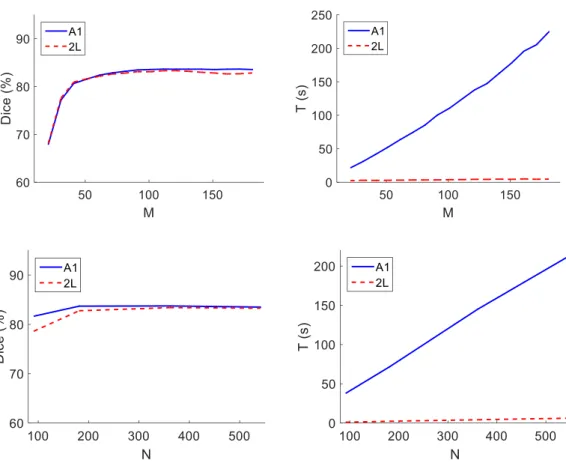
Fig. 7. Computational performance: (left) the Dice coefficient and (right) the time spent per 100 iterations, T. In the top row, different values of M were tested, using N = 361 (fixed); in the bottom row, different values of N were tested, using M = 120 (fixed).
4.2.1 Computational performance
The computational complexity of the algorithms A1 and 2L depends on two main parameters:M and N, which determine the size of the edge map. These two parameters influence the performance of the proposed approaches both in terms of time spent per 100 iterations, T, and the quality of the segmentations.
The computational performance of the algorithm was evaluated on the dataset D1, on a MATLAB implementation, running on an Intel (R) Core(TM) i7 CPU at 2.93 GHz.
Fig. 7 shows the Dice coefficient and T for different values of M = {20, 30, . . . , 170, 180}, assumingN = 361 fixed, andN ={91,181,361,541}, assuming M = 120 fixed. It is possible to see in the top right corner that, as expected, the complexity A1 depends linearly on the value ofM, whereas the complexity of L2 does not depend on M. Consequently, the time required to run A1 may be significantly larger than that of L2. However, in terms of segmentation quality, the difference between these two approaches is almost negligible. The value of the Dice coefficient reaches a plateau at around M = 100, with the
Table 1
Statistical evaluation of the 2L algorithm in the segmentation of the LV in 33 sequences of cardiac MRI [11], using the GT masks to create the edge maps.
Dice (%) AV (mm) 2L+AU 97.6 (0.9) 0.3 (0.4)
Fig. 8. Examples of segmentations in non-circular LV shapes.
maximum being achieved at M = 120. Larger values of M only decrease the speed of the overall algorithm, without affecting its accuracy. Regarding the number of columns in the edge map, N, both algorithms have a similar behavior: the time per 100 iterations increases linearly with N, although at very different scales, while the Dice coefficient stabilizes for N ≥181, with a maximum reached at N = 361.
4.2.2 Segmentation using the GT
In this section, the proposed algorithm is applied to segment binary masks that correspond to the GT segmentations, in dataset D1. Contrary to real world images, in this analysis the edge associated to the LV border is well defined and the valleys of the edge map accurately follow the desired path.
There is an inherent bias to this experiment, but the goal of this analysis is twofold. First, it establishes an upper bound on the accuracy of the algorithm.
Since the edge maps obtained with the GT masks are ideal, the performance of the algorithm in the corresponding cardiac MRI images will always be worse.
Second, it allows studying if the algorithm is able to deal with all the different LV shapes (e.g., elliptical LVs).
Table 1 shows the statistical results obtained with the 2L+AU algorithm. It is
possible to see that, given the GT masks, the algorithm has a very high average Dice coefficient and low average distance to the GT, which mean it is able to fit the LV border very accurately. From these results, we can conclude that the performance of the algorithm depends almost exclusively on the ability of the edge map to capture the LV border.
Fig. 8 further illustrates that the algorithm is able to segment images in which the LV border is not exactly circular, even though that is a premise of the proposed approach.
The penalty coefficient, η, used to determine the optimal path along the edge map (recall equation (14)) allows us to control the flexibility of the model to fit non-circular shapes. Ifη is set too high, it may constrain the segmentation too much and prevent the algorithm from following the desired path, thus it will not be able to fit non-circular shapes. On the other hand, if this value is too low, it could lead to a segmentation with an irregular border. In these studies, the penalty coefficient was empirically chosen to be η = 0.05, which grants enough flexibility to the model while ensuring that the segmentation border is smooth, and this was the value used in the remaining tests.
Additionally, a different experiment was also performed, in which the ground truth binary masks were segmented using a circle. The idea of this study is to further validate the underlying assumption that the LV has a circular shape, by evaluating the quality of the segmentations using circles. In order to fit a circle to the ground truth, we computed the centroid of the ground truth mask as the estimate of the circle center, and the average distance of the ground truth points to the centroid as the estimated radius. The corresponding segmentations have an average Dice coefficient of 92.3%±2.6%, and an average distance of 1.3 mm±0.5 mm. These results demonstrate that a circle is a good approximation of the LV border in most images.
4.2.3 Influence of the initialization
As mentioned above, the proposed algorithm requires an initial guess of the center and radius of the LV in the image it is trying to segment. This is a po- tential source of variability, since different initializations may lead to different results. This section aims to determine how dependent the performance of the algorithm is on the initialization.
To illustrate the influence of the initialization, a specific example image was randomly chosen (see Fig. 9 top left corner). In order to determine the influ- ence of the initial guess of the LV center, we fixed the initial guess of R and performed the segmentation for different values of center c, around the true LV center. More specifically, the A1+AU algorithm was applied 61×61 times and, in each test, the initial guess of c was one of the 61×61 pixels inside
Dice (a)
(b) (c)
(d)
(a)
(b) (c)
(d)
(a) (b)
(c) (d)
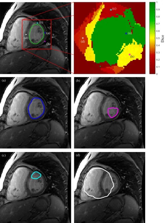
Fig. 9. Performance of A1+AU for different initial guesses of the LV center. The initial guesses are each of the pixels inside the red square (top left), and the Dice coefficient of the corresponding segmentation is shown on the top right. (a) to (d) show different examples of the segmentations obtained when choosing the initial center identified by the corresponding label and color in the top images. The green contour (top left) is the GT.
the red square shown in Fig. 9 top left corner. The corresponding Dice coeffi- cient is shown in Fig. 9 top right corner, with a color code in which greener
Fig. 10. Statistical evaluation of the influence of the initial guess of the LV center in the algorithm’s accuracy.
1stiteration 2nditeration 3rditeration 4thiteration Initial guess
Fig. 11. Example of the segmentation obtained (red) with an erroneous initial guess of the LV radius, along several iterations of A1+AU. The green contour is the GT.
is better. It is possible to see that the algorithm performs better when initial- ized close to the true LV center, as expected. However, the figure also shows that there are distinct regions within which the accuracy of the segmentation is homogeneous. Furthermore, the green area is very large, which means that the algorithm is able to converge to the correct segmentation even if the initial guess of the center is not very accurate. The four bottom plots in Fig. 9 show examples of the segmentation obtained by initializing the center within four different regions (identified by the letter (a)-(d) in the top row) It is possible to see that in (b)-(d), the algorithm is either misguided by papillary muscles (as shown in (b) and (c)) or by the right ventricle (as shown in (d)). For the entire (green) region to which (a) belongs, the algorithm is able to obtain the correct segmentation of the LV.
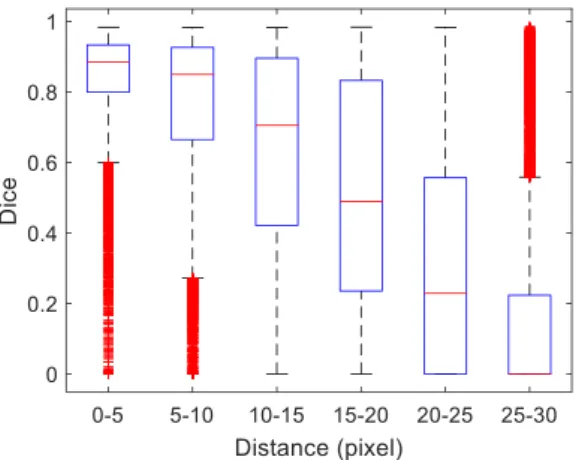
A statistical evaluation was also performed to determine the quality of the segmentations as the initial guess of the center moves away from the true LV center. The results are depicted in the boxplots in Fig. 10, where we compare the Dice coefficient against increasingly larger initial center guess errors. The distance between the true center and the initial guess was divided into 6 bins:
0-5, 5-10, 10-15, 15-20, 20-25, 25-30 pixels. For each bin, random perturbations to the true center were generated so that each of the 5011 images in the dataset D1 was tested using 5 different initial center guesses with the corresponding
Table 2
Statistical evaluation of the proposed approaches in the dataset D1, with 33×20 volumes. For each algorithm, the table shows the results for all the segmentations (dashed entries in the “% Good” column) and excluding segmentations with AV
>5 mm. Each entry shows the mean value and standard deviation.
Dice (%) AV (mm) % Good VolumeTime (s) A1 82.2 (9.1) 2.8 (1.4) -
11.2 85.6 (6.1) 2.2 (0.6) 87.2
A1+AU 83.5 (9.1) 2.6 (1.3) -
55.4 86.1 (7.0) 2.1 (0.6) 89.7
2L+AU 82.8 (11.2) 2.7 (1.7) -
1.5 85.9 (8.3) 2.1 (0.7) 88.8
error. Thus, each bin corresponds to a total of 5×5011 = 25055 examples.
The figure shows that the algorithm achieves good segmentation results with errors up to 10 pixels. For larger errors, its performance rapidly decreases, because the segmentation tries to fit other edges in the image, as shown in the examples in Fig. 9.
Regarding the initial guess of the LV radius, R, the tests showed that the algorithm is very robust. It is able to accurately segment the LV even if the initial guess of R is very different from the true LV radius, with an average Dice coefficient of 91.54±0.06 for initial radii R = 4, . . . ,34 mm. This is ensured by limiting the values of rmax and rmin, used to convert the image to polar coordinates (recall equation (3)). Since we know that the LV radius is anatomically bounded (e.g., within the values rmin >1 mm and rmax <34 mm in the dataset D1), it is possible to constrain the size of the segmentation, despite having erroneous estimates ofR. Fig. 11 shows an example of an initial guess of R = 4 mm and its evolution throughout the iterations of algorithm A1+AU, where it is possible to see that the algorithm converges to the correct segmentation despite the wrong initial estimate.
4.2.4 Segmentation results for two cardiac MRI datasets
Table 2 shows the statistical results of the three approaches discussed in this work for the dataset D1. Regarding the accuracy of the segmentations, all the approaches have a similar performance. Nonetheless, the performance of A1+AU is better than 2L+AU, which in turn is better than A1. However, if we also take into account the time required to segment each volume, then the 2L+AU approach is considerably more attractive than the other two.
Statistical results of the proposed segmentations are compared to state-of-
Table 3
Performance comparison with state-of-the-art approaches. Dashed entries mean the information was not provided.
Dataset D1 [11]
Dice (%) AV (mm) % Good SequenceTime (s) Ehrhardt [42] 1 83 (NA) 1.8 (0.7) - -
Santiago [43] 79 (8) 3.5 (1.4) - -
O’Brien [44] - 1.4 (0.2) - -
Andreopoulos [11] - 1.4 (1.3) - 456
Pham [45] 2 90.5 (2.6) - - -
2L+AU 85.9 (8.3) 2.1 (0.7) 88.8 30 Dataset D2 [41]
Dice (%) AV (mm) % Good SequenceTime (s) Huang [46] 89 (4) 2.2 (0.5) 79.2 -
Gopal [47] 84 (4) 3.7 (0.6) - -
Avendi [36] 94 (2) 1.8 (0.4) 96.7 - Queir´os [48] 90 (5) 1.8 (0.5) 92.3 11 Constantinides [49] 86 (5) 2.4 (0.6) 80 60
Hu [50] 89 (3) 2.2 (0.4) 91 154
Liu [51] 88 (3) 2.4 (0.4) 91.2 129 Uzunbas [52] 82 (6) 3.0 (0.9) - 45
Jolly [20] 88 (4) 2.3 (0.6) 95.6 60 2L+AU 86.0 (6.3) 2.6 (0.7) 82.1 30
1 uses only 25 of the 33 sequences available for testing.
2 uses only 10 of the 33 sequences available for testing.
the-art methods in Table 3 for the two datasets. These methods use other approaches to obtain the segmentations, namely image-based methods [46,50, 51], deformable models with or without shape information [11,20,42–45,47–49, 52], and a combined deep learning and deformable model approach [36]. The results in Table 3 show that the proposed method is able to achieve comparable results to all the other state-of-the-art approaches. It is important to note that the proposed system uses very little shape information compared to most of the other approaches.
Fig. 12 shows a comparison between the medical parameters based on the
Fig. 12. Comparison of the medical parameters: ESV (top), EDV (middle) and EF (bottom). Each plot compares the parameters obtained using the proposed segmen- tations and the GT. The left plots show the correlation graph and the right plots show the Bland-Altman comparison.
proposed segmentations and based on the GT in the dataset D2. This figure shows that they are highly correlated, although there is a systematic under- estimation of the ESV and EDV that is linear with the increase in volume.
Dice
Fig. 13. Discriminated evaluation of the segmentation of each volume in the dataset (33 patients × 20 frames). The colormap indicates the Dice coefficient, in which green pixels correspond to good segmentation and red to poor segmentations.
Since the behavior is similar in both phases of the cardiac cycle, the result- ing EF is very similar to the EF obtained with the GT segmentations. This means that even though the volumes are underestimated with the proposed segmentations, the method is able to accurately compute the corresponding EF, which can then be used to diagnose cardiac function.
Fig. 13 shows the Dice coefficient obtained using L2+AU for each of the 33×20 volumes in the dataset. Most of the volumes are very well segmented and the poorer segmentations are easily identified by the few red pixels in the figure.
This image also shows that the proposed algorithm performs better during the diastolic phase (approximately frames 1-5 and 11-20) than in the systolic phase (6-10), which is expected since the edges along the LV border are clearer in these frames. Most segmentation failures (red pixels in Fig. 13) were either caused by the presence of papillary muscles (see bottom right example in Fig.
14), or because the segmentation was pulled towards the LV’s outer border (see bottom left examples in Fig. 14). These cases are hard to segment using an edge-based approach, since the strongest edge does not correspond to the desired border. This is a drawback of many of the works shown in Table 3, since they also rely on edge detection.
Another issue to consider is that the proposed approach segments the volume slices sequentially. Therefore, when one of the slices is incorrectly segmented, the error may propagate to the following slices. While using 3D shape con- straints may be tempting, performing the segmentation in a 2D setting also avoids issues due to misaligned slices, which are common in cardiac MRI [53].
In these cases, updating the center and radius estimates has significant advan- tages, since it allows the algorithm to recover from segmentation errors. The example in Fig. 15 illustrates this advantage. The figure shows the segmenta-
Fig. 14. Examples of segmentations obtained using 2L+AU (in red) and comparison with the GT (green). Each image shows one slice from a particular patient.
Dice
A1A1+AU
Fig. 15. Comparison between A1 (top row) and A1+AU (bottom row). Each column shows a slice of the volume, from the basal slice (left) to the apex (right); the red contour is obtained using the automatic algorithm and the green is the GT. The last column shows a 3D view of the volume segmentations and the corresponding color-coded Dice coefficient.
tion of a particular volume using A1 (top row) and A1+AU (bottom row). In both cases, the initial guess of the center and radius in the basal slice (left) is the same. It is possible to see that the A1 algorithm is not able to accu- rately segment the LV. Even though the error is not significant, it escalates to meaningless segmentations in the following slices. By using the automatic update scheme, the A1+AU algorithm is able to recover from these poorer initial estimates.
5 Discussion
The goal of the proposed method is to provide fast and accurate segmentation of the LV in cardiac MRI. The results showed in the previous section provide several insights about the proposed algorithm.
First, it shows that the proposed approach, in particular the 2L+AU algo- rithm, is able to obtain good and very fast segmentations of the LV (see Table 2). This is relevant from the cardiologist’s perspective since it means we are able to provide a good estimate of the LV border with very little human in- put. Thus, the total effort required to analyze these images is significantly reduced. Even in specific cases where the proposed segmentation needs refine- ment, using this algorithm in the clinical setup is still an improvement over the traditional manual approach, because the automatic segmentations can be obtained quickly.
Second, the results shown in Section 4.2.2 also demonstrate that the underlying assumption that the LV has a circular shape is not only valid but also strong enough to provide good segmentations. On one hand, fitting a circle to the ground truth segmentations leads to an average Dice coefficient of 92.3% and an average distance of 1.3 mm, whereas applying the proposed approach to the ground truth masks leads to an average Dice coefficient of 97.6% and an average distance of 0.3 mm. On the other hand, we also show that the algorithm is flexible enough to allow the model to fit non-circular shapes (e.g., elliptical LV), as shown in the examples in Fig. 8.
Third, the proposed method is able to achieve good segmentation accuracies even when the initial guess of the LV center is as far as 10 pixels away from the true LV center. For larger errors, the performance of the algorithm starts to decrease because it tends to be attracted to other anatomical structures in the image.
Finally, the proposed algorithm is able to provide cardiologists with fast seg- mentations of the LV, which has not been a concern of most works in the literature. Instead, many of the state of the art works focus on proposing complex frameworks that typically require a significant amount of training data and disregard the high running-time figures [11,36,52,54].
6 Conclusions
A fast methodology for the segmentation of the LV in cardiac MRI is pre- sented in this work. This approach is built under the assumption that the LV
segmentation in each slice has approximately a circular shape. We propose to transform the original MR slice into an edge map in polar coordinates, whose valleys roughly follow the LV border. Then, the delineation of the LV contour is obtained using a DP approach. The results show that this approach is able to achieve good results, and is able to compete with other state-of-the-art ap- proaches, most of which use more complex shape assumptions. The proposed approach is also able to segment a whole volume in 1.5 seconds, i.e., it pro- vides fast and accurate segmentations that would significantly reduce the time spent by cardiologists in this laborious task.
The drawback of the proposed algorithm is the fact that it relies on edge de- tection to identify the position of the LV border. Although this is a common approach in the literature, the outer wall of the LV and the presence of pap- illary muscles may misguide these algorithms. Therefore, future work should focus on using a more robust approach to compute the edge map, instead of relying on edge detection. Also, it would be advantageous to replace the manual initialization step by an automatic approach, such as using the Hough transform for circles or following the approach used in [20], as this would lead to a fully automatic method.
7 Acknowledgments
This work was supported by the PhD grant [SFRH/BD/87347/2012] and FCT grants [UID/EEA/50009/2013] and [PTDC/EEIPRO/0426/2014].
References
[1] C. Jenkins, S. Moir, J. Chan, D. Rakhit, B. Haluska, T. H. Marwick, Left ventricular volume measurement with echocardiography: a comparison of left ventricular opacification, three-dimensional echocardiography, or both with magnetic resonance imaging, European heart journal 30 (1) (2009) 98–106.
[2] J. Dias, J. Leit˜ao, Wall position and thickness estimation from sequences of echocardiographic images, IEEE Transactions on Medical Imaging 15 (1) (1996) 25–38.
[3] J. S. Marques, P. Pina, Crater delineation by dynamic programming, IEEE Geoscience and Remote Sensing Letters 12 (7) (2015) 1581–1585.
[4] C. Petitjean, J.-N. Dacher, A review of segmentation methods in short axis cardiac MR images, Medical image analysis 15 (2) (2011) 169–184.
[5] V. Tavakoli, A. A. Amini, A survey of shaped-based registration and segmentation techniques for cardiac images, Computer Vision and Image Understanding 117 (9) (2013) 966–989.
[6] A. Suinesiaputra, B. R. Cowan, A. O. Al-Agamy, M. A. Elattar, N. Ayache, A. S. Fahmy, A. M. Khalifa, P. Medrano-Gracia, M.-P. Jolly, A. H. Kadish, et al., A collaborative resource to build consensus for automated left ventricular segmentation of cardiac MR images, Medical image analysis 18 (1) (2014) 50–62.
[7] R. Van der Geest, E. Jansen, V. Buller, J. Reiber, Automated detection of left ventricular epi-and endocardial contours in short-axis MR images, in:
Computers in Cardiology 1994, IEEE, 1994, pp. 33–36.
[8] X. Lin, B. R. Cowan, A. A. Young, Automated detection of left ventricle in 4D MR images: experience from a large study, in: International Conference on Medical Image Computing and Computer-Assisted Intervention, Springer, 2006, pp. 728–735.
[9] E. Nachtomy, R. Cooperstein, M. Vaturi, E. Bosak, Z. Vered, S. Akselrod, Automatic assessment of cardiac function from short-axis MRI: procedure and clinical evaluation, Magnetic resonance imaging 16 (4) (1998) 365–376.
[10] J. Cousty, L. Najman, M. Couprie, S. Cl´ement-Guinaudeau, T. Goissen, J. Garot, Segmentation of 4D cardiac MRI: Automated method based on spatio- temporal watershed cuts, Image and Vision Computing 28 (8) (2010) 1229–1243.
[11] A. Andreopoulos, J. K. Tsotsos, Efficient and generalizable statistical models of shape and appearance for analysis of cardiac MRI, Medical Image Analysis 12 (3) (2008) 335–357.
[12] A. Katouzian, A. Prakash, E. Konofagou, A new automated technique for left-and right-ventricular segmentation in magnetic resonance imaging, in:
Engineering in Medicine and Biology Society, 2006. EMBS’06. 28th Annual International Conference of the IEEE, IEEE, 2006, pp. 3074–3077.
[13] D. Geiger, A. Gupta, L. A. Costa, J. Vlontzos, Dynamic programming for detecting, tracking, and matching deformable contours, IEEE Transactions on Pattern Analysis and Machine Intelligence 17 (3) (1995) 294–302.
[14] A. Lalande, L. Legrand, P. M. Walker, F. Guy, Y. Cottin, S. Roy, F. Brunotte, Automatic detection of left ventricular contours from cardiac cine magnetic resonance imaging using fuzzy logic, Investigative radiology 34 (3) (1999) 211–
217.
[15] J. Fu, J. Chai, S. T. Wong, Wavelet-based enhancement for detection of left ventricular myocardial boundaries in magnetic resonance images, Magnetic resonance imaging 18 (9) (2000) 1135–1141.
[16] J.-Y. Yeh, J. Fu, C. Wu, H. Lin, J. Chai, Myocardial border detection by branch- and-bound dynamic programming in magnetic resonance images, Computer methods and programs in biomedicine 79 (1) (2005) 19–29.
[17] X. Qian, Y. Lin, Y. Zhao, J. Wang, J. Liu, X. Zhuang, Segmentation of myocardium from cardiac MR images using a novel dynamic programming based segmentation method, Medical physics 42 (3) (2015) 1424–1435.
[18] N. Liu, S. Crozier, S. Wilson, F. Liu, B. Appleton, A. Trakic, Q. Wei, W. Strugnell, R. Slaughter, R. Riley, Right ventricle extraction by low level and model-based algorithm, 27th Annual IEEE Engineering in Medicine and Biological Society 27 (2005) 677–680.
[19] P. Soille, Morphological image analysis: principles and applications, Springer Science & Business Media, 2013.
[20] M. Jolly, Fully automatic left ventricle segmentation in cardiac cine MR images using registration and minimum surfaces, The MIDAS Journal-Cardiac MR Left Ventricle Segmentation Challenge 4.
[21] Y. Cai, A. Islam, M. Bhaduri, I. Chan, S. Li, Unsupervised Freeview Groupwise Cardiac Segmentation Using Synchronized Spectral Network, IEEE transactions on medical imaging 35 (9) (2016) 2174–2188.
[22] M. Kass, A. Witkin, D. Terzopoulos, Snakes: Active contour models, International journal of computer vision 1 (4) (1988) 321–331.
[23] W. Zhou, Y. Xie, Interactive medical image segmentation using snake and multiscale curve editing, Computational and mathematical methods in medicine 2013.
[24] Y. Wu, Y. Wang, Y. Jia, Segmentation of the left ventricle in cardiac cine MRI using a shape-constrained snake model, Computer Vision and Image Understanding 117 (9) (2013) 990–1003.
[25] C. Xu, J. L. Prince, Snakes, shapes, and gradient vector flow, IEEE Transactions on image processing 7 (3) (1998) 359–369.
[26] M. Santarelli, V. Positano, C. Michelassi, M. Lombardi, L. Landini, Automated cardiac MR image segmentation: theory and measurement evaluation, Medical engineering & physics 25 (2) (2003) 149–159.
[27] H.-Y. Lee, N. C. Codella, M. D. Cham, J. W. Weinsaft, Y. Wang, Automatic left ventricle segmentation using iterative thresholding and an active contour model with adaptation on short-axis cardiac MRI, IEEE Transactions on Biomedical Engineering 57 (4) (2010) 905–913.
[28] D. Nguyen, K. Masterson, J.-P. Vall´ee, Comparative evaluation of active contour model extensions for automated cardiac MR image segmentation by regional error assessment, Magnetic Resonance Materials in Physics, Biology and Medicine 20 (2) (2007) 69–82.
[29] Y. Liu, G. Captur, J. C. Moon, S. Guo, X. Yang, S. Zhang, C. Li, Distance regularized two level sets for segmentation of left and right ventricles from cine- MRI, Magnetic resonance imaging 34 (5) (2016) 699–706.
[30] M. Alessandrini, T. Dietenbeck, O. Basset, D. Friboulet, O. Bernard, Using a geometric formulation of annular-like shape priors for constraining variational level-sets, Pattern Recognition Letters 32 (9) (2011) 1240–1249.
[31] K. Punithakumar, I. B. Ayed, I. G. Ross, A. Islam, J. Chong, S. Li, Detection of left ventricular motion abnormality via information measures and bayesian filtering, IEEE Transactions on Information Technology in Biomedicine 14 (4) (2010) 1106–1113.
[32] J. Folkesson, E. Samset, R. Y. Kwong, C.-F. Westin, Unifying statistical classification and geodesic active regions for segmentation of cardiac MRI, IEEE Transactions on Information Technology in Biomedicine 12 (3) (2008) 328–334.
[33] N. Paragios, A level set approach for shape-driven segmentation and tracking of the left ventricle, IEEE transactions on medical imaging 22 (6) (2003) 773–776.
[34] G. Carneiro, J. C. Nascimento, A. Freitas, The segmentation of the left ventricle of the heart from ultrasound data using deep learning architectures and derivative-based search methods, IEEE Transactions on Image Processing 21 (3) (2012) 968–982.
[35] G. Carneiro, J. C. Nascimento, Combining multiple dynamic models and deep learning architectures for tracking the left ventricle endocardium in ultrasound data, IEEE transactions on pattern analysis and machine intelligence 35 (11) (2013) 2592–2607.
[36] M. Avendi, A. Kheradvar, H. Jafarkhani, A combined deep-learning and deformable-model approach to fully automatic segmentation of the left ventricle in cardiac MRI, Medical image analysis 30 (2016) 108–119.
[37] R. Szeliski, Computer vision: algorithms and applications, Springer Science &
Business Media, 2010.
[38] M. Isard, A. Blake, Active contours, Springer-Verlag Berlin Heidelberg, 1998.
[39] J. C. Nascimento, J. S. Marques, Adaptive snakes using the EM algorithm, IEEE Transactions on Image Processing 14 (11) (2005) 1678–1686.
[40] D. P. Bertsekas, Dynamic programming and optimal control, Athena Scientic, 2005.
[41] P. Radau, Y. Lu, K. Connelly, G. Paul, A. Dick, G. Wright, Evaluation framework for algorithms segmenting short axis cardiac MRI, The MIDAS Journal-Cardiac MR Left Ventricle Segmentation Challenge 49.
[42] J. Ehrhardt, T. Kepp, A. Schmidt-Richberg, H. Handels, Joint multi-object registration and segmentation of left and right cardiac ventricles in 4D cine MRI, in: SPIE Medical Imaging, International Society for Optics and Photonics, 2014, pp. 90340M–90340M.
[43] C. Santiago, J. C. Nascimento, J. S. Marques, 2D Segmentation using a robust active shape model with the EM algorithm, IEEE Transactions on Image Processing 24 (8) (2015) 2592–2601.
[44] S. P. O’Brien, O. Ghita, P. F. Whelan, A Novel Model-Based 3D+Time Left Ventricular Segmentation Technique, IEEE Transactions on Medical Imaging 30 (2) (2011) 461–474.
[45] V.-T. Pham, T.-T. Tran, K.-K. Shyu, L.-Y. Lin, Y.-H. Wang, M.-T. Lo, Multiphase B-spline level set and incremental shape priors with applications to segmentation and tracking of left ventricle in cardiac MR images, Machine vision and applications 25 (8) (2014) 1967–1987.
[46] S. Huang, J. Liu, L. C. Lee, S. K. Venkatesh, L. L. San Teo, C. Au, W. L.
Nowinski, An image-based comprehensive approach for automatic segmentation of left ventricle from cardiac short axis cine mr images, Journal of digital imaging 24 (4) (2011) 598–608.
[47] S. Gopal, D. Terzopoulos, A unified statistical/deterministic deformable model for LV segmentation in cardiac MRI, in: International Workshop on Statistical Atlases and Computational Models of the Heart, Springer, 2013, pp. 180–187.
[48] S. Queir´os, D. Barbosa, B. Heyde, P. Morais, J. L. Vila¸ca, D. Friboulet, O. Bernard, J. Dhooge, Fast automatic myocardial segmentation in 4D cine CMR datasets, Medical image analysis 18 (7) (2014) 1115–1131.
[49] C. Constantinid`es, E. Roullot, M. Lefort, F. Frouin, Fully automated segmentation of the left ventricle applied to cine MR images: description and results on a database of 45 subjects, in: Engineering in Medicine and Biology Society (EMBC), 2012 Annual International Conference of the IEEE, IEEE, 2012, pp. 3207–3210.
[50] H. Hu, H. Liu, Z. Gao, L. Huang, Hybrid segmentation of left ventricle in cardiac MRI using gaussian-mixture model and region restricted dynamic programming, Magnetic resonance imaging 31 (4) (2013) 575–584.
[51] H. Liu, H. Hu, X. Xu, E. Song, Automatic left ventricle segmentation in cardiac MRI using topological stable-state thresholding and region restricted dynamic programming, Academic radiology 19 (6) (2012) 723–731.
[52] M. G. Uzunba¸s, S. Zhang, K. M. Pohl, D. Metaxas, L. Axel, Segmentation of myocardium using deformable regions and graph cuts, in: Biomedical Imaging (ISBI), 2012 9th IEEE International Symposium on, IEEE, 2012, pp. 254–257.
[53] C. Santiago, J. C. Nascimento, J. S. Marques, A new ASM framework for left ventricle segmentation exploring slice variability in cardiac MRI volumes, Neural Computing and Applications (2016) 1–12doi:10.1007/
s00521-016-2337-1.
[54] T. Anh Ngo, G. Carneiro, Fully automated non-rigid segmentation with distance regularized level set evolution initialized and constrained by deep-structured inference, in: Proceedings of the IEEE Conference on Computer Vision and Pattern Recognition, 2014, pp. 3118–3125.
![Fig. 4. 2-loop algorithm [2]. The blue line depicts the solution of A1 with initial position r(1) = r min ; the red line depicts the solution of A1 on the reordered edge map with initial position r 0 (1) = r(N/2); the green dashed line represents the groun](https://thumb-eu.123doks.com/thumbv2/123dok_br/19418920.0/13.892.132.733.105.679/algorithm-depicts-solution-position-solution-reordered-position-represents.webp)