MSEi i the mean square error of the ith response surface êi predicted standard deviation for the ith response 2. This obstacle is partially overcome by [4], considering the response surface of the first principal component as objective function and the following components as constraints. Then, each MMSEi index will be considered as a new objective function that can be optimized according to the routine and parameters of the NBI method.
The variance equation can be found by writing a response surface model for the absolute value of the residual εikl of the. 14 eigenvalues of the variance-covariance (Ʃ) or correlation (R) matrices of yp with Z(yp) its standardized value [23]. Σˆ is the variance-covariance matrix of the residuals of the fitted models, and Fm,n-r-m(α) is the upper (100α)-th percentile of an F-distribution with m and n-r-m degrees of freedom.
Development of proposed method
The fitness of the model can be improved using a multivariate least squares algorithm (MWLS), as described in Eq. 13), with a diagonal matrix of weights (Wnxn) defined as the reciprocal of the squared Mahalanobis distance (MD) established for the residuals of the first OLS models, as shown in Eq. Where: MD in this case represents the Mahalanobis distance of the residues; epx1. represents the vector of the residuals for the pOLS models in the nth run; Σˆpp denotes the variance-covariance matrix of the residuals of the p-response surface models. The confidence ellipsoid for each predicted Pareto point will be found correctly substituting Eq. 12), as the following statements will be detailed. 15), MSE(FA)i represents the “mean square error” of the ith rotated factor score surface model, FAi(x).
T , can be obtained by individual optimization or can be settled according to the decision maker's preferences as well as the goals of the rotated factor score equations. Assume that there exists a confidence ellipsoid for each solution in a given Pareto frontier, with the vector of expected means considered as its centroid and a variance-covariance matrix written in terms of the estimated variance functions. 13), Wnxn is a diagonal matrix of weights whose elements are defined as the inverse of squared Mahalanobis Distance (MD) established for the residuals of the first OLS models, Eq.
Therefore, in order to choose the most appropriate solution according to the decision maker's preference, it is necessary to evaluate the degree of importance of the elements used to distinguish Pareto solutions, i.e. The Mahalanobis distance (MD) and the ellipse volume (V). . Adapting the Mahalanobis Distance (MD) to measure the process mean vector "shift" it is possible to write:. 22), the parameter y represents the covariance between f1(x) and f2(x), where (Spxp) represents their variance-covariance matrix. 23), the parameter p represents the number of dimensions (or variables) considered in the problem, n is the number of degrees of freedom for the error term, α is the significance level and Γ(.) represents the gamma function [25] .
Discrimination between MD and V can be established using the concept of Fuzzy decision maker [28, 29], in which membership functions are constructed for attributes according to the arbitrary degree of preference manifested by the decision maker. To execute this step, it is necessary to parameterize the Utopia and Nadir values for each function, calculating the memberships and ordering them according to the Fuzzy logic scenario, in the interval [0, 1].
Material and methods
19 In this context, it is desirable that functions have the smallest Mahalanobis distance, as well as the smallest confidence ellipse volume. Fuzzy decision maker (μT) is defined as the weighted sum of membership functions considered [5], assuming the form of Eq. Then the better Pareto solution will be the one with the highest Fuzzy decision maker value (μT).
It is worth mentioning that in this paper, displacement of means will be considered more important than variances, with an arbitrated ratio of around 85/15. After correlation analysis of the data, both mean and variance data are transformed into equimax rotated factor scores to create the uncorrelated models. Although any rotation method could be used in this case, "Equimax" will promote factor with similar associated eigenvalues.
Then, these functions are simultaneously optimized by applying the NBI method, resulting in a complete Pareto frontier (Step 4). In sequence, a confidence ellipse is established for each point of the Pareto frontier according to the corresponding mean vector and the variance-covariance matrix obtained during the optimization. Finally, for each considered solution, the volumes of the confidence ellipses are calculated, as well as the Mahalanobis Distance between the mean and the corresponding target (Step 5).
These two measures thus form a Fuzzy decision maker (step 6), which in turn allows the choice of the most appropriate parameters for the process, depending on the interest of the indicated researcher. By applying the concept of non-overlapping trust regions, the most suitable Pareto optimal solution is found (step 7).
Modeling of Mean and Variance: Starting with DOE, it is generated a central composite response surface design considering process variables (factors) and their respective
Further, the dimensionality of the optimization problem is reduced by agglutinating the Fa objective functions into the MSE-FA functions (Step 3). 21 correlation analysis is performed to investigate the existence of dependence between responses (experimental data). It is worth noting that anomalous behavior in the residuals can be detected using graphical approaches and can indicate the presence of non-normal response variables.
In addition to the expected correlation between the original responses, heteroscedastic models will generally present a significant correlation between the expected values and the variances. Therefore, the PCFA approach can be used to disentangle the response variables in an uncorrelated data set. In FA it is functions and then avoiding correlated variables in subsequent optimization.
In the FA, it is possible for data to be separated independently, that is, effectively representative of mean and variance for each process response. The factor score of each response is modeled by OLS with the same RSM design.
Agglutination of FA of Mean and Variance into a MSE metric: The pairs of factor scores of mean and variance models for each process response are agglutinated into a
Numerical examples and results
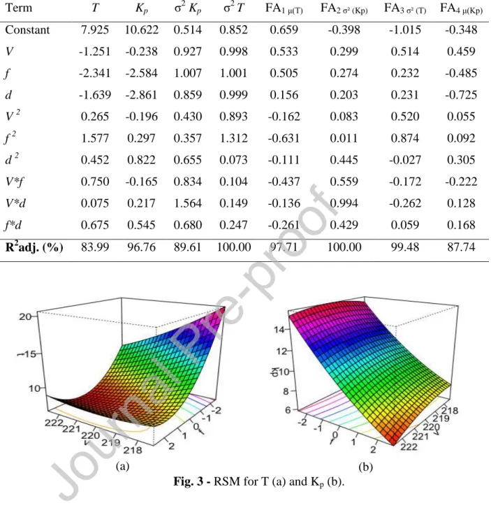
Tool flank wear measurements (VBmax) were taken by an optical microscope and the tool break point was used as criteria for end life. Continuing with the Pearson's correlation analysis, a positive and significant correlation between T and Kp is observed around 0.776, with P-value equal to 0.000. By extracting four factors using principal component analysis and Equimax rotation, the following PCFA analysis is obtained (Table 4).
Therefore, it is possible to verify that FA1 is the best representative of μ(T) with a negative correlation. When we write the MSE-FA index for vehicle life, for example, we notice that both (FA1 - TFA1)2 and FA3 must be minimized, which implies that MSE-FA can also be minimized. Following the procedure established in step 3, the objectives for the MSE functions are calculated using the GRG algorithm with xTx≤ρ2 as a unique constraint.
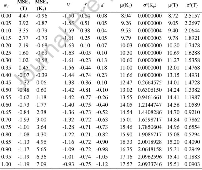
To complete the step 4 procedure, the multi-objective nonlinear optimization algorithm from Eq. 20) is iteratively performed using GRG for different weights that form the Pareto frontier for MSE(FA)1 and MSE(FA)2 (with respect to Kp) shown in Figure 31. As a complement to the routine from step 5, the volume of each ellipse is calculated with p. 26) is used for two responses (T and Kp) m = 2, which has a CCD design with 18 observations (n) and the response models have 9 coefficients (r) each, except for the constant term, as in Eq. 27). Then, with a weight of 85/15 among the membership functions, the best value for the Fuzzy decision maker is 0.943 (higher).
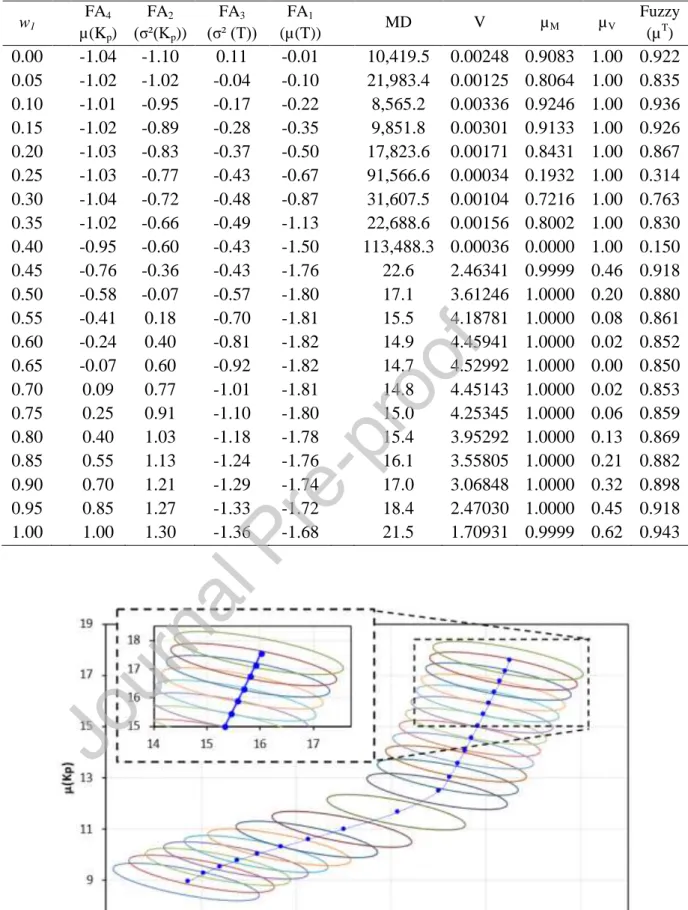
Finally, after removing the overlapping ellipses, the filtered Pareto frontier shown in Fig. , Kp, 2( )T and 2(Kp), extracting four factors using principal component and Equimax rotation (Table 10). From Table 10 it is possible to verify that FA4 replaces μ(T) and presents a negative correlation with this variable; therefore, minimizing FA4 leads to maximizing tool life; FA3 is positively correlated with σ2 (T), then minimizing it reduces the variance of tool life.
After all the confidence ellipses are plotted (Fig. 10), it is possible to analyze and remove those Pareto points that overlap.

Conclusions
As a matter of comparison, the multiobjective optimization of this second case study was repeated with several different available algorithms: (a) the NBI-MMSE method as described in Eq. 7), (b) the traditional NBI in four dimensions (NBI*), (c) the method of weighted sums with MMSE functions (WSUM-MMSE*), (d) the global criterion method (MCG-MMSE*) and Bow homotopy length (AHL-MMSE*), both with multivariate mean squared error function of Eq. From an optimization perspective, such separation allows the influence of the weights to be better transferred to the objective functions. The second advantage is related to the capacity of the rotation method to negate the conflict between the sense of optimization of the original variable and the response surface model of the factor scores.
This feature, which was not observed in the PCA score, allowed the definition of features with the same degree of importance before the weighting process promoted by the interactions of the NBI algorithm. The use of 95% confidence ellipses was found to be an appropriate approach to filter the initial Pareto-optimal solutions, reducing the number of alternatives for posterior evaluation. In the case of multi-objective optimization of the turning process of AISI 52100 hardened steel performed with CC6050 mixed ceramic inserts, the minimum process cost, the maximum tool life and minimum variance for both reactions were achieved with a cutting speed equal to 220.4 m/min, feed equal to 0.209 mm/rev and depth of cut equal to 0.340 mm.
It is worth noting that the large difference between T and Kp in the numerical cases is due to differences in the type of inserts and in the cost of the steels used. 2] Paiva, A.P., Costa, S.C., Paiva, E.J., Balestrassi, P.P., Ferreira, J.R., Multi-objective optimization of pulsed gas metal arc welding process based on weighted scores of principal components, Intl. Silva et al., Normal boundary crossing method based on principal components and Taguchi's signal-to-noise ratio applied to the multi-objective optimization of the 12L14 free-machining steel turning process, Int.
Paiva, A multiobjective optimization model for machining quality in AISI 12L14 steel turning process using fuzzy multivariate mean square error, Precis. Balestrasi, A normal boundary crossing approach for robust multi-feedback optimization of bottom surface roughness.