2 2-mean curvature for vertical graphs over M

Constructions of H _r -hypersurfaces, barriers and Alexandrov Theorem in IH ⁿ × IR

Maria Fernanda Elbert and Ricardo Sa Earp March 2, 2014

Abstract

In this paper, we are concerned with hypersurfaces in IH×IR with constant r-mean cur- vature, to be calledH_r-hypersurfaces. We construct examples of completeH_r-hypersurfaces which are invariant by parabolic screw motion or by rotation. We prove that there is a unique rotational strictly convex entire H_r-graph for each value 0 < H_r ≤ ⁿ⁻_n^r. Also, for each value H_r > ⁿ⁻_n^r, there is a unique embedded compact strictly convex rotational H_r-hypersurface. By using them as barriers, we obtain some interesting geometric results, including height estimates and an Alexandrov-type Theorem. Namely, we prove that an embedded compact H_r-hypersurface in IHⁿ×IR is rotational (Hr>0).

Introduction

The r-mean curvature, Hr, of an n-hypersurface is defined as the normalized r-symmetric function of the principal curvatures (see section 1 for precise definitions). In this paper, we are concerned with hypersurfaces with constant r-mean curvature, to be called Hr-hypersurfaces.

Although we sometimes work in a more general setting, we are particularly interested in the case the ambient is the product space IHⁿ×IR, where IHⁿ denotes the hyperbolic space. Throughout the paper, we establish some key equations for the theory. For instance, in Section 7, we deduce a suitable divergence formula for the r-mean curvature of a vertical graph over M inM ×IR.

We start, in Sections 2, 3 and 4, by exploiting the geometry of the hypersurfaces with constant H2 in IHⁿ ×IR. In Section 5, 6 and 7, we deal with the general case r > 2. When n = 2, we recall that H₂ is the extrinsic curvature K_ext of the surface.

We classify the complete Hr-hypersurfaces that are invariant by parabolic screw motion with H_r = 0 (see Theorem (5.2)) and we classify some of the complete ones which are invariant by rotation, for Hr > 0 (see Theorem (5.6)). Surprisingly, they show a strong analogy with the study of the mean curvature case in IHⁿ ×IR. For the mean curvature, the behavior of the

Keywords and sentences: r-mean curvature, Alexandrov Theorem,Hr-hypersurfaces, barriers, entire vertical graphs, complete horizontal graphs.

2000 Mathematical Subject Classification: 53C42, 53A10, 53C21.

The authors are partially supported by CNPq of Brazil.

rotational H-hypersurface, H >0, depends on the value of H and we distinguish the cases of H greater or less than the critical value ⁿ⁻_n¹ (see [B-SE2] and [E-SE]). For the r-mean curvature, Hr > 0, the same happens for the value ⁿ⁻_n^r. We should also notice that similarly to what happens for the mean curvature, there is a unique rotational strictly convex entire vertical graph for each constant value 0 < Hr ≤ ⁿ⁻_n^r. Also, for each constant value Hr > ⁿ⁻_n^r, there is a unique embedded compact strictly convex rotational Hr-hypersurface. Both are unique up to vertical or horizontal translations (see Theorem (5.6)). The dependence on r and n is a distinguishing point from the theory of Hr-hypersurfaces in IHⁿ×IR (Hr >0) from that of the euclidean or hyperbolic spaces, where the critical points are 0 and 1, respectively (See [P]).

By using some of the constructed examples as barriers, we were able to obtain some interest- ing results (see Section 6). For instance, we prove that there is no compact without boundary immersion in IHⁿ×IR with prescribed r-mean curvature function H_r : M −→ (0,ⁿ⁻_n^r], n > r.

We also obtaina priori height estimates for compact immersions of IHⁿ×IR with boundary in a slice and with prescribed r-mean curvature functionHr :M −→(0,ⁿ⁻_n^r], n > r. An interesting question is if we could obtain a height estimate for the case H_r > ⁿ⁻_n^r and we ask: Would the maximum height of a compact graph with boundary in a slice with Hr = constant > ⁿ⁻_n^r be given by half of the total height of the compact rotational corresponding example? In fact, J. A.

Aledo, J. M. Espinar and J. A G´alvez (see [A-E-G]) proved that is true for H-graph in IH²×IR.

In [E-G-R], J.M. Espinar, J.A. G´alvez and H. Rosenberg address the case of surfaces with positive extrinsic curvature in some 3-dimensional product spaces. In particular, they show that a complete immersion in IH²×IR with H2 =constant >0 (i.e.,r=n= 2) is a rotational sphere (see [E-G-R, Theorem 7.3]). For n >2, our Example (4.4) shows that there exist entire graphs with H₂ > 0 in IHⁿ×IR. It is natural to ask what kind of complete H_r-immersions, r = n, Hr>0, we can find. As one can see below, we have partial answers to this question.

In Theorem (6.6), we prove an Alexandrov-type Theorem (see [A] for the classical result) for compact embedded Hr-hypersurfaces in IHⁿ×IR, i.e., we characterize the embedded compact Hr-hypersurfaces in IHⁿ × IR, Hr > 0. Precisely, if Hr > 0, we prove that a compact Hr- hypersurface embedded in IHⁿ×IR is rotational (which is classified). Here, we notice that we only have compact rotational Hr-hypersurfaces for Hr > ⁿ⁻_n^r (see Theorem (5.6)). In space forms, an Alexandrov-type result for the r-mean curvatures were obtained by N.J. Korevaar in [K] and by S. Montiel and A. Ros in [M-R].

On the other hand, for Hr > ⁿ⁻_n^r, there exist no entire rotational Hr-graph (see Theorem (5.6)). It is interesting to investigate the complete Hr-hypersurface for this case. We ask, for instance: Is there a noncompact complete embedded Hr-hypersurface in IHⁿ×IR, Hr > ⁿ⁻_n^r, with only one end. If n=2, in [E-G-R, Theorem 7.2], the authors proved that if Kext > 0 (or H > 1/2), there is no properly embedded Kext-surface (or H-surface) in IH² ×IR with finite topology and one end.

We have then seen that for H_r > ⁿ⁻_n^r, the only compact embedded immersion is a rotational n-sphere and that there exist no entire rotational Hr-graph. We ask if for the particular case r =n we have the same behavior of the caser =n = 2, that is :

Question: Is a complete immersion in IHⁿ ×IR, with Hr = constant > 0 and r = n a

rotational n-sphere?

1 Preliminaries

LetMⁿ be an oriented Riemannian n-manifold, ¯Mⁿ⁺¹ be an oriented Riemannian manifold and X : Mⁿ → M¯ⁿ⁺¹ be an isometric immersion. For each p ∈ M, let A : T_pM → T_pM be the linear operator associated to the second fundamental form of X and k1, ..., kn be its eigenvalues corresponding to the eigenvectors e1, . . . , en. The r-mean curvature of X is then defined by

H_r(p) = 1

n r

X

i1<...<ir

k_i1...k_ir = 1

n r

S_r(p),

whereS_r is ther-symmetric function ofk₁, ..., k_n. With this notation, H₁ is the mean curvature, H, of the immersion and Hn is the Gauss-Kronecker curvature. The Newton tensors associated to X are inductively defined by

P0 = I,

P_r= S_rI−A◦P_r−1, r >1 and will be useful to recall that

(1) (r+ 1)S_r+1 = trace(P_rA),

(2) Pr−1(ei) = ∂Sr

∂ki

(ei) and that

(3) trace(Pr) = (n−r)Sr.

For details and other properties, we suggest the paper [B-C] from L. Barbosa and G. Colares.

If Hr+1 = 0 we say that the immersion is r-minimal. In this context, the classical minimal immersions would be the 0-minimal ones.

We say that an immersion X is strictly convex (convex) at p ∈M if ki(p) >0 (respectively ki(p) ≥0) for all i = 1, . . . , n, with respect to the normal orientation at p. In the literature, a strictly convex point is usually called an elliptic point.

Although we sometimes work in a more general setting, we are particularly interested in the case ¯M = IHⁿ×IR, where IHⁿ denotes the hyperbolic space. We start by the case r= 2 and we recall that when n= 2, S2 =H2 is the extrinsic curvature Kext of the surface.

2 2-mean curvature for vertical graphs over M

Let M =Mg denote a Riemannian n-manifold with metric g and consider on ¯M =M ×IR the product metric h,i=g+dt², where t is a global coordinate for IR.

If uis a real function defined over Ω⊂M, the setG={(p, u(p))∈M×IR|p∈Ω} is called the vertical graph of u, or more simply, the graph of u. We denote by X : Ω ⊂ M → M ×IR the natural embedding of GinM ×IR. If u is C² and if we choose the orientation given by the upward unit normal, namely N =

−^∇_W^gu,_W¹

, it is proved in [E1, Formula (3)] that

(4) A(v) =∇^gv

∇gu W

, for allv ∈T M,

where∇^g and∇^gare, respectively, the connection and the gradient ofM andW =q

1 +|∇^gu|²g. Let Ric_g(v₁, v₂) = trace(z→R_g(v₁, z)v₂) denote the Ricci tensor of M. Then, the following proposition holds.

Proposition 2.1. The 2-mean curvature H2 of the graph G is given by (5) 2S2 =n(n−1)H2 =divg

P1∇gu W

+Ricg

∇gu W ,∇gu

W

,

where divg means the divergence in M.

Proof:

By (1) and (4) we have

2S₂ = trace

z→P₁∇^gz

∇gu W

.

Claim:

(6) trace (z →P1∇^gzv) = trace (z → ∇^gz(P1v)) +Ricg

v,∇gu W

.

The proposition will be proved by taking v = ^∇_W^gu in the latter. In order to prove the claim, we follow the proof of [E1, Lemma (3.2)] without assuming Ricg = 0. We sketch it here for completeness.

By the definition of the curvature Rg and by (4) we have (7) ∇^gv(A(z))− ∇^gz(A(v)) = R(z, v)

∇gu W

+A([v, z]).

Let p ∈ M and let {v_i}i be an orthonormal basis in a neighborhood of p in M which is geodesic at p, that is, such that ∇^gvjvi(p) = 0. Let v =X

i

aivi. Since {vi}i is geodesic at pwe have

trace(z →P1∇^gz(v))(p) = trace z→X

i

z(ai)P1(vi)

! (p).

On the other hand,

trace(z → ∇^gz(P1(v))(p) = trace(z →X

i

z(ai)P1(vi))(p) +X

i

aitrace(z → ∇^gz(P1(vi)))(p).

Putting things together we have

trace(z →P1∇^gz(v)(p) = trace(z → ∇^gz(P1(v)))(p)−X

i

aitrace(z → ∇^gz(P1(vi)))(p).

The proof will be completed if we prove that

trace (z → ∇^gz(P1(vi))) (p) =−Ricg(vi,∇^gu W ).

The latter holds as can be seen below, where in the third equality we use (7).

trace (z → ∇^gz(P1(vi))) (p) = trace (z → ∇^gz(S1(vi)−A(vi))) (p)

= trace (z →z(S1)vi) (p)−trace (z → ∇^gz(A(vi))) (p)

= vi(S1)(p)−trace (z → ∇^gvi(A(z))) + trace z →Rg(z, vi)) ^∇_W^gu (p)

= v_i(S₁)(p)−trace (z → ∇^gvi(A(z)))−trace z →R_g(v_i, z) ^∇_W^gu (p)

= −Ricg(vi,^∇_W^gu).

We remark that equation (5), that gives the 2-mean curvature of the graph, is elliptic iff P₁ is positive definite. If S2 > 0, a standard argument shows that it is elliptic (see, for instance, [E1, proof of Lemma 3.10]).

From now on, in this section, we consider the particular case whereMⁿ ⊂IRⁿand we denote by (x1, x2, . . . , xn) the (Euclidean) coordinates of M. On M, we consider the metric given by

g = 1

F² h., .i,

where h., .i= (dx₁²+. . .+dx_n²) is the euclidean metric. For such a particular M, Proposition (2.1) reads as follows.

Proposition 2.2. The 2-mean curvature of the graph of u when M is as above is given by

(8) 2S2 =n(n−1)H2 =F²div

P1∇u W

+(2−n)F hP1∇u,∇Fi

W +Ricg

∇gu W ,∇gu

W

. Here, div, ∇, and ||.|| denote quantities in the Euclidean metric and W can be written as W =p

1 +F²||∇u||² .

Sketch of the Proof:

Let {ei}ⁱ be an orthonormal local field of M in the metric h., .i. Then

divg

P1∇^gu W

=X

i

ei,∇^gei

P1

∇^gu W

=X

i

ei,∇^gei

P1

F²∇u W

. Now we use the relation between the connections and gradients of the two conformal metrics g and h., .i, Proposition (2.1) and some computation to obtain the result.

Remark 2.3. An expression relating the Ricci Tensor of two conformal metrics can be obtained in [S-Y, page 183]. By using it for our case, we have that

Ricg(vi, vj) = (n−2)Fij

F + ∆F

F −(n−1)|∇F|² F²

δij,

where ∆ denotes the laplacian in the euclidean metric and Fij denotes the second derivative of F. Doing this, one can express formula (8) in terms of the euclidean metric only.

Now we look forward to expressing the 2-mean curvature in the coordinates (x1, x2, . . . , xn).

For this, let X(x1, x2, . . . , xn) = (x1, x2, . . . , xn, , u(x1, x2, . . . , xn)) be the natural parametriza- tion of G and let {e1, . . . , en} be an orthonormal basis of vector fields of M in the euclidean metric. We write Xi =dX(ei) = (ei, ui). Then, a computation gives the following proposition.

Proposition 2.4. Let [I] = [Iij]and [II] = [IIij] denote the matrices of the first and the second fundamental forms of the (isometric) embedding X in the basis {ei}i. Let [I]⁻¹ = [I^ij] be the inverse matrix of [I]. Then we have

Iij = δij

F² +uiuj

IIij =−∇¯^XiN, Xj

= uij

W + 1

F W

"

uiFj +ujFi − X

m

umFm

! δij

# ,

and

I^ij =F²δij −F⁴uiuj

W²

where we write ui anduij for the corresponding first and second derivative of the function uand

∇¯ for the connection of M ×IR.

Remark 2.5. We can use the last proposition in order to re-obtain [E-SE, formula(1.3)].

In the basis {ei}ⁱ, we can express the matrix of A as

(9) [A] = [I^ij]×[IIij]

and in order to obtain an explicit expression for the 2-mean curvature of G in the coordinates (x1, x2, . . . , xn), one can use (1). The computation, in the general case, is a tough job but can be done by adapting the proof given by M. L. Leite in [L2, Proposition (2.2)] and the result is the following.

Proposition 2.6. The 2-mean curvature H2 of the graph G of u considering in M ⊂ IRⁿ the metric g = _F¹2 h,i and the coordinates (x1, x2, . . . , xn) is given by

(10)

S2

W⁴

F⁴ =n(n−1)H2

W⁴

F⁴ = X

i<j

W²−F²(u²_i +u²_j)

V_{ii} V_{ij}

V_{ji} V_{jj}

− 2F²X

i<k

uiuk

X

j6=i,k

V_{ik} V_{ij}

V_{jk} V_{jj}

,

where V_{ij} =uij+ 1 F

"

uiFj +ujFi− X

m

umFm

! δij

#

=IIij.W and the indices vary in {1, ..., n}.

In this paper, we are in fact interested in the case where M = IHⁿ is the hyperbolic space.

ChoosingF conveniently, we will be able to deal with different models for IHⁿ. For future use, we point out that by using that the Ricci curvature of IHⁿ is−(n−1) we can rewrite the expression (8) for this case as

(11) 2S2 =n(n−1)H2 =F²div

P1∇u W

+(2−n)F hP1∇u,∇Fi

W −(n−1)F²

∇u W

2

.

Of course, one can use the formula of Remark (2.3) to obtain (11).

3 Examples of complete H

-graphs in IH

× IR

In this section, we consider the half-space model for IHⁿ, that is, we consider IHⁿ={x= (x1, . . . , xn−1, xn=y)∈IRⁿ|y >0} endowed with the metric

dx²₁+. . .+dx²_n

F² = dx²₁+. . .+dx²_n

y² .

Searching for examples, here we consider for each (l₁, . . . , l_n−1) ∈ IRⁿ⁻¹, the graph G given by

(12) t=u(x1, . . . , xn−1, y) =λ(y) +l1x1+. . .+ln−1xn−1

and we have the following.

Proposition 3.1. The 2-mean curvature H2 of the graph G of t =λ(y) +l1x1+. . .+ln−1xn−1

is given by

(13) 2S2

y² = n(n−1)H2

y² =



− y

l²+ (n−1) ˙λ² W²





′

+ (n−1)(n−3) ˙λ²−l²

W² ,

where l² =l12+. . .+ln−12 and W² = 1 +y²l²+y²λ˙². Sketch of the Proof:

By using Proposition (2.4) and (9) we can obtain the matrix [A] and,a fortiori, [P₁]. Then, we obtain the result by computing formula (11).

Remark 3.2. By using Proposition (2.6) for graphs given by (12) we obtain the equation

2S2W⁴ = (n−1)(n−4) ˙λ²y²+(n−1)(n−2) ˙λ⁴y⁴+(n−1)(n−2) ˙λ²y⁴l²+2 ˙λλy¨ ³[(2−n)l²y²−(n−1)]−2l²y², that turns out to be equivalent to (13). The latter can also be obtained by using (1).

We want to solve equation (13) for some particular data finding then some interesting graphs with constant 2-mean curvature. For simplifying purposes, we introduce in (13) the variable z =l² + (n−1) ˙λ² obtaining

2S2

y² =− z W²y_′

+ (n−3) z

W² + (2−n) l² W², or equivalently,

(14) 2S2

yⁿ⁻¹ =− z

W²y⁴⁻ⁿ_′

+ (2−n)l²y³⁻ⁿ W² .

We recall that a parabolic translation can be identified with a horizontal Euclidean transla- tion in this model for IHⁿ. Then, whenl = 0, the graphGgiven by (12) is invariant by parabolic translation. When l 6= 0, the parabolic translation is composed with a vertical translation and we say that Gis invariant by parabolic screw motion.

We notice that in IHⁿ × IR we can also define the notion of a horizontal graph, y=g(x1, . . . , xn−1, t), of a real and positive function g.

We first deal with the case l= 0 andS₂ = 0, and we obtain the following classification result.

Theorem 3.3. (1-minimal hypersurfaces inIHⁿ×IR invariant by parabolic translations) Despite the slice, 1-minimal vertical graphs invariant by parabolic translations are, up to vertical translations or reflection, of the following type:

a) If n= 2, λ(y) =cln(y), for all y >0 and for c >0.

b) If n >2, λ(y) = _n−²₂arcsin(^y

n−22

c ), for a positive constant c and y ∈ (0, cⁿ⁻²² ).

The function λ(y) in a) gives rise to an entire vertical graph. The functionλ(y) in b) generate a family of non-entire horizontal 1-minimal complete graphs in IHⁿ×IR invariant by parabolic translations. The asymptotic boundary of each graph of this family is formed by two parallel (n−1)-planes.

Proof:

Equation (14) for l = 0 and S₂ = 0 yields z

W²y⁴⁻ⁿ =d, for a constant dthat must be non-negative.

Replacing the values for z and W and integrating we obtain, up to reflection, λ(y) =

Z y 0

√d ξⁿ⁻⁴²

p(n−1)−d ξⁿ⁻²dξ.

If n = 2 we obtain a) with c=q

d

1−d and if n >2, we set c=q

n−1

d and we obtain b).

The function λ(y) given by b) is increasing in the interval (0, cⁿ⁻²²) and is vertical at y = cⁿ⁻²² . Since the induced metric in the yt-plane is euclidean, a simple computations shows that the Euclidean curvature is finite at this point and strictly positive at this point. If we set t0 =λ

cⁿ⁻²²

, we can then glue together the graph t=λ(y) with its reflection given by 2t0−λ(y)

in order to obtain a horizontal 1-minimal complete graph invariant by parabolic screw motion defined over {(x₁, . . . , x_n−1, t) ∈ IHⁿ⁻¹ ×IR | 0 ≤ t ≤ 2t₀}. The asymptotic boundary of this example is formed by two parallel hyperplanes.

Remark 3.4. Recalling that when n = 2, S₂ is the extrinsic curvature of the surface, we see that each solution of Theorem(3.3) a)gives rise to an entire graph with null extrinsic curvature.

By considering the result given in [E-SE, Proposition (4.1)], one can see that this solution has constant mean curvature H = ¹₂^√_1+c^c 2. Then, the solution λ(y) = cln(y), c ∈ IR, is an entire graph with null extrinsic curvature and constant mean curvature |H|< ¹₂. We wonder if this is the only example of an entire graph with null extrinsic curvature and constant mean curvature in IH²×IR.

Question: Are there any entire graph with null extrinsic curvature and constant mean curvature in IH²×IR other than λ(y) =cln(y), c∈IR ?

We could handle to find solutions for equation (14) for some values of n, l and S₂. We do not aim to exhaust the cases here but we choose some particular data in order to present some interesting examples.

Example 3.1. [Graphs with null extrinsic curvature inIH²×IRinvariant by parabolic screw motion]

Equation (14) for n= 2, l6= 0 and S2 = 0 yields z

W²y² =d which implies that d >0 and gives

λ =± Z y

∗

pc−ξ²l²

ξ dξ, where c= d

1−d >0.

The integration gives, up to vertical translations or reflection, the explicit solution λ =−√

cln(√ c+p

c−l²y²) +√

cln(ly) +p

c−l²y², for y∈(0, rc

l).

Example 3.2. [Entire H₂-graphs in IHⁿ×IR invariant by parabolic translations, 0< H₂ <

n−2

n , n >2]

Equation (14) for l= 0 and H2 =k 6= 0 yields n(n−1)k

yⁿ⁻¹ =− z

W²y⁴⁻ⁿ_′ , which, for n >2, gives

z W² =

n(n−1)k n−2

1 y². The latter implies that k >0 and can be written as

((n−2)−nk) ˙λ² = (nk) 1 y².

Then, we must have 0< k < ⁽ⁿ⁻_n²⁾. Integration gives, up to vertical translations, the solution λ =cln(y), c ∈IR, y >0.

In [E-G-R, Theorem 7.3], the authors proved that, when n = 2, a complete immersion with H2 =constant >0 is a rotational sphere. In contrast, when n >2, the last example shows that there exist entire graphs with H2 =constant >0.

Remark 3.5. One can easily see that when n = 2 or l = 0, we can obtain explicit solutions of (14) by integration. For each case, a careful analysis of the behavior should be taken.

4 Examples of rotational H

-hypersurfaces in IH

× IR

Now, we search for rotational hypersurfaces of IHⁿ×IR withH₂ =constantand we use the ball model of the hyperbolic space IHⁿ (n ≥2), i.e., we consider

IHⁿ={x= (x1, . . . , xn)∈IRⁿ|x²₁+. . .+x²_n≤1} endowed with the metric

gIH := dx²₁+. . .+dx²_n

F² = 1

F² h., .i, where F =

1−|x|² 2

.

We notice that in [E-G-R, Section 5], the authors classify the complete rotational surfaces in IH²×IR with constant positive extrinsic curvature. With our method, we could re-obtain their examples (see Example (4.3) below). In [L1], [P], [C-P] and references therein, one can find examples of rotational hypersurfaces with constant Hr in space forms as well as classification results.

In the vertical plane V := {(x1, . . . , xn, t) ∈ IHⁿ×IR|x1 = . . . = xn−1 = 0} we consider a generating curve (tanh(ρ/2), λ(ρ)), for positive values of ρ, the hyperbolic distance to the axis IR.

For our purpose, we define a rotational hypersurface in IHⁿ×IR by the parametrization X :

( IR+×Sⁿ⁻¹ → IHⁿ×IR

(ρ, ξ) → (tanh(ρ/2), λ(ρ)).

The normal field to the immersion and the associated principal curvatures will be given by N = (1 + ˙λ²)^−1/2( −λ˙

2 cosh²(ρ/2)ξ,1),

k1=k2 =...=kn−1 = cotgh (ρ) ˙λ(1 + ˙λ²)^−1/2 and kn= ¨λ(1 + ˙λ²)^−3/2.

(See [B-SE1, Section 3.1] with a slight modification writing functions in terms of ρinstead oft).

Then, the 2-mean curvature

(ⁿ₂)H2 =S2 = X

i1<i2

ki1ki2

is given by

(15) nH2

(sinhⁿ⁻¹(ρ)) cosh(ρ) = ∂

∂ρ

"

sinhⁿ⁻²(ρ) λ˙² 1 + ˙λ²

!#

.

By setting I(ξ) =Rξ 0

(sinh⁽ⁿ⁻¹⁾(s))

cosh(s) ds and integrating twice we obtain, up to vertical translation or reflection,

(16) λ(ρ) = Z ρ

∗

s nH2I+d

sinh⁽ⁿ⁻²⁾(ξ)−(nH₂I+d)dξ, where the constant d comes from the first integration.

Now we set

p(ξ) =nH₂I+d and q(ξ) = sinh⁽ⁿ⁻²⁾(ξ)−(nH₂I+d) = sinh⁽ⁿ⁻²⁾(ξ)−p(ξ)

and we write

λ(ρ) = Z ρ

∗

sp(ξ) q(ξ)dξ.

We notice that we must have p(ξ) ≥0 and q(ξ) >0. We also notice that when d 6= 0, λ could not be defined for ρ= 0, since, in this case, ^p(0)_q(0) =−1.

Differentiation gives

λ˙ ≥0,

˙

p=nH2

sinh⁽ⁿ⁻¹⁾(ξ) cosh(ξ) ,

(17) q˙= sinhⁿ⁻³(ξ) cosh(ξ)

(n−2) cosh²(ξ)−nH2sinh²(ξ)

= sinhⁿ⁻³(ξ) cosh³(ξ)

1− nH2

(n−2)tgh²(ξ)

and

¨λ= 1 2

q p

1/2

˙ pq−pq˙

q²

= 1 2q²

q p

1/2

sinhⁿ⁻³(ξ)

cosh(ξ) [nH2sinhⁿ(ξ)−(n−2) cosh²(ξ)p], forξ >0.

Now, exploring (16) and analyzing the behavior of the functions p and q we highlight some interesting examples of rotational H2-hypersurfaces in IHⁿ×IR and their geometric properties.

Example 4.1. [The slice]

We easily see that the slice, λ =constant, is a solution of (15) for H2 = 0 and any dimension.

Example 4.2. [1-minimal cones in IH²×IR]

Setting n= 2 andH₂ = 0 in (15) we obtain the solution λ(ρ) =±

r d

1−d ρ, 0< d <1.

Thus, we see that the cone λ(ρ) = cρ, c∈ IR, ρ >0, is a 1-minimal surface in IH² ×IR, i.e., a surface with null extrinsic curvature. In euclidean coordinates, we can write them as

t = 2c arctgh (p

x²+y²), c∈IR, x²+y² <1.

Example 4.3. [Compact rotational surface with positive extrinsic curvature in IH²×IR]

Setting n= 2, d= 0 and H₂ >0, the expression in (16) reads as follows

λ(ρ) = Z ρ

0

s

2H2ln(cosh(ξ)) 1−(2H₂ln(cosh(ξ))) dξ

and we must have ρ < ρo := arcosh (e^2H12). We want to analyze the convergence of the integral atρ0. By using that ln(cosh(ξ)) and tgh (ξ) are increasing functions we have, for alla ∈(0, ρ),

Z ρ0

a

s 2H2ln(cosh(ξ))

1−(2H2ln(cosh(ξ))) dξ ≤ Z ρ0

a

s 1

1−(2H2ln(cosh(ξ))) dξ

≤ 1

2H2tgh (a) Z ρ0

a

2H2tgh (ξ)

p1−(2H2ln(cosh(ξ))) dξ.

By setting v(ξ) = 2H2ln(cosh(ξ)) and using the inequalities above we can see that

Z ρ0

a

s 2H₂ln(cosh(ξ))

1−(2H2ln(cosh(ξ))) dξ ≤ 1 2H2tgh (a)

Z 1 v(a)

r 1 1−v dv and then the integral is convergent at ρ0 and λ(ρ0) is well defined.

Now, we use (17) to see that, for ξ >0,

˙

p >0, q <˙ 0 and ¨λ = 1 2

q p

1/2

[pq˙ −pq˙ q² ]>0.

Bringing all together we see that λ is increasing and strictly convex in the interval (0, ρ₀) and is vertical and assume a finite value at ρ=ρ0.

Since the induced metric in the ρt-plane is euclidean, a simple computation shows that the Euclidean curvature is finite at this point and strictly positive at this point. If we sett0 =λ(ρ0), we can then glue together the graph t=λ(y) with its reflection given by

2t0−λ(y) in order to obtain a compact rotational surface.

We now choose d = 0 and n > 2 in the expression (16). We notice that, for this case,

ξlim→0

p(ξ)

q(ξ) = 0 then we can set ^p(0)_q(0) = 0 and we have

(18) λ(ρ) =

Z ρ 0

s nH2I

sinh⁽ⁿ⁻²⁾(ξ)−nH₂I dξ.

We also notice that, with these conditions, there is no solution for H2 <0, since we would have

p(ξ)

q(ξ) <0. Then, it remains to treat the case H2 >0.

Lemma 4.1. The function λ given by (18), for H2 >0 and n >2:

i) is increasing.

ii) satisfies λ >¨ 0, for all ξ > 0.

iii) satisfies λ= ^√H₂²ρ²+o(ρ³), near 0.

In particular, the corresponding hypersurface is strictly convex.

Proof:

i) is clear. We proceed with the proof of ii).

For all ξ > 0, we write the last equation in (17) as λ¨= 1

2q² q

p 1/2

sinhⁿ⁻³(ξ) cosh(ξ) S(ξ), where S(ξ) = nH2sinhⁿ(ξ)−(n−2) cosh²(ξ)p. A computation gives

S(ξ) = 2 sinh(ξ) cosh(ξ)(nH˙ 2sinhⁿ⁻²(ξ)−(n−2)p).

Now, we set R(ξ) = nH2sinhⁿ⁻²(ξ)−(n−2)pand we have S(ξ) = 2 sinh(ξ) cosh(ξ)R(ξ).˙ We easily see that

R(ξ) = (n˙ −2)nH2

sinhⁿ⁻³(ξ)

cosh(ξ) >0 for all ξ >0.

Then, we can see thatR, anda fortioriS, vanish atξ = 0 and is positive forξ >0. This finishes the proof.

The formula in iii) is the Taylor approximation for λ near ξ= 0.

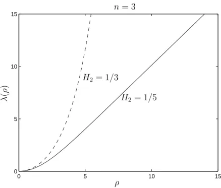
Example 4.4. [Entire rotational strictly convex H₂-graph in IHⁿ×IR with 0 < H₂ ≤ ⁿ⁻_n², n >2]

We have q(0) = 0 and λ= ^√H₂²ρ²+o(ρ³) near 0. Since tgh (ξ)<1, the expression for ˙q in (17) gives that ˙q > 0 for ξ > 0. Then, the generating curve is given by a function λ(ρ) defined for ρ >0. By applying Lemma (4.1) it follows that the generating curve is strictly convex.

0 5 10 15 0

5 10 15

ρ

λ(ρ)

n= 3

H2 = 1/3

H2 = 1/5

Figure 1: Entire rotational strictly convex H2-graph with 0< H2 ≤ ⁿ⁻_n²,n = 3

0 5 10 15

0 5 10 15

ρ

λ(ρ)

n= 4

H2 = 1/2

H2 = 1/3

Figure 2: Entire rotational strictly convex H₂-graph with 0< H₂ ≤ ⁿ⁻_n²,n = 4

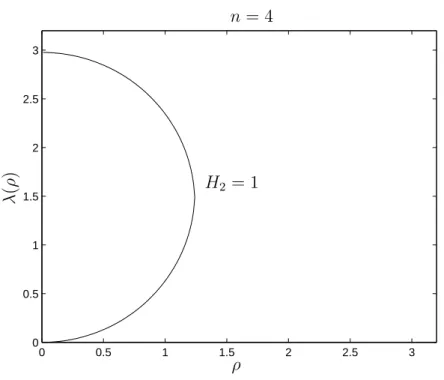
Example 4.5. [Compact embedded strictly convex rotational H₂-hypersurface in IHⁿ×IR with H₂> ⁿ⁻_n², n >2]

We have q(0) = 0 and as before, near 0, λ has the following behavior λ=

√H2

2 ρ²+o(ρ³).

We observe that the asymptotic behavior of q(ξ) when ξ tends to infinity is as follows q(ξ) = e^(n−2)ξ

2ⁿ⁻²

(1 +e^−2ξ)⁽ⁿ⁻²⁾−( nH2

n−2) +O(e^−2ξ)

.

Then, we can see that whenH2 > ⁿ⁻_n² >0,q(ξ) becomes negative whenξtends to infinity. Also, the behavior of the function tgh (ξ) gives, by using the expression for ˙qin (17), that ˙qis positive near zero, vanishes at ξ = arctgh (q

n−2

nH2) and becomes negative later. This shows that q is positive near 0, attains a maximum at arctgh (q

n−2

nH2), has a positive root ρ0 > arctgh (q

n−2 nH2) and is negative for ξ > ρ0.

Then λ(ρ) is defined for ρ ∈ [0, ρ0) and at ρ0 we have nH2I(ρ0) = sinh⁽ⁿ⁻²⁾(ρ0). Also, since nH2I(ξ) is increasing we obtain

Z ρ0

0

s nH2I

sinh⁽ⁿ⁻²⁾(ξ)−nH₂Idξ≤ Z ρ0

0

s

sinh⁽ⁿ⁻²⁾(ρ0)

sinh⁽ⁿ⁻²⁾(ξ)−sinh⁽ⁿ⁻²⁾(ρ₀)dξ By setting v = _sinh(ρ^sinh(ξ)

0) we see that Z ρ0

0

s nH2I

sinh⁽ⁿ⁻²⁾(ξ)−nH2Idξ ≤ Z 1

0

sinh(ρ0) q

1 +v²sinh²(ρ0)

.(vⁿ⁻²−1)^−1/2dv≤ Z 1

0

v⁻¹(vⁿ⁻²−1)^−1/2dv.

Since R

v⁻¹(vⁿ⁻²−1)^−1/2 = _n−²₂arctan(vⁿ⁻²−1)^1/2+constant, we conclude that the integral converges to a finite value t0 =λ(ρ0) at ρ0.

Then, we see that for each value of H2 greater that ⁿ⁻_n², we obtain that λ is increasing and strictly convex in the interval (0, ρ0) and is vertical and assume a finite value at ρ=ρ0.

Since the induced metric in the ρt-plane is euclidean, a simple computation shows that the Euclidean curvature is finite and strictly positive at this point. If we sett₀ =λ(ρ₀), we can then glue together the graph t=λ(y) with its reflection given by

2t0−λ(y)

in order to obtain an embedded compact rotational surface.

0 0.5 1 1.5 2 2.5 3 0

0.5 1 1.5 2 2.5 3

ρ

λ(ρ)

n= 4

H2 = 1

Figure 3: Embedded compact strictly convex rotational H2-hypersurface with H2 > ⁿ⁻_n²,n = 4 In order to highlight the geometric properties of the examples with d = 0, we notice that careful analysis of (18) gives the following proposition that we will need later.

Proposition 4.2. For fixed n, the profile curves of the rotationalH2-hypersurfaces obtained by (18) satisfy:

i) For a fixed ρ, λ increases when H₂ increases.

ii) For H2 > ⁿ⁻_n², we have that ρ0 tends to infinity when H2 tends to ⁿ⁻_n².

iii) λ(ρ) → 0 uniformly in compacts subsets of [0,∞] when H2 → 0. This means that when H₂ →0, the rotationalH₂-hypersurfaces converge to the slice, uniformly in compact subsets of IHⁿ× {0}.

5 Generalizations for H

-hypersurfaces, r > 2

In this section, we give an insight into the case r > 2. Again, by adapting the proof of [L2, Proposition (2.2)] given by M. L. Leite, we obtain

Proposition 5.1. The r-mean curvature Hr of the graph G of u considering in M ⊂ IRⁿ the metric g = _F¹2 h,i and the coordinates (x₁, x₂, . . . , x_n) is given by

(19)

Sr

W^r+2

F^2r = X

j1<...<jr

W²−F²(u²_j1 +. . .+u²_jr)

V_{j1j1} V_{j1j2} . . . V_{j1jr} V_{j1j2} V_{j2j2} . . . V_{j2jr}

. . . . V_{j1jr} V_{j2jr} . . . V_{jrjr}

− 2F²X

i<k

uiuk







 X

j2,...,jr6=i,k

V_{ik} V_{ij2} . . . V_{ijr} V_{j2k} V_{j2j2} . . . V_{j2jr}

. . . . V_{jrk} V_{jrj2} . . . V_{jrjr}







 ,

whereV_{ij} =uij + 1 F

"

uiFj+ujFi− X

m

umFm

! δij

#

=IIij.W and the indices vary in{1, ..., n}. Forr = 1, formula (19) is equivalent to [SE-T, formula (3)] and forr= 2 it reduces to formula (10) of Proposition (2.6). We can use it to construct many examples of Hr-hypersurfaces. For instance, we can consider the half-space model for IHⁿand the graphGof differentiable functions of the form t = v(x1) in order to obtain hypersurfaces with Hr = 0. Now, as in Section 3, we consider the graph G of functions of the form t = u(x1, . . . , xn−1, y) = λ(y). We have the following.

Theorem 5.2. (Hypersurfaces with Hr= 0 in IHⁿ×IR invariant by parabolic translations) Despite the slice, vertical graphs G with Hr = 0 are, up to vertical translations or reflection, of the following types:

i) If n=r, λ(y) =cln(y), for all y >0 and for c >0.

ii) If n > r, λ(y) = _n−^r_rarcsin(^y

n−r r

c ), for a positive constant c and y ∈ (0, c^n−rr ).

The function λ(y) in a) gives rise to an entire vertical graph. The functionλ(y) in b) generate a family of non-entire horizontal (r −1)-minimal complete graphs in IHⁿ ×IR invariant by parabolic translations. The asymptotic boundary of each graph of this family is formed by two parallel (n−1)-planes.

Proof:

For G, we have the following Vij =−λ(y)˙

y δij, for i, j ≤n, Vnn = ¨λ(y) + λ(y)˙ y

and

W² = 1 +y²λ˙²(y).

The last proposition then yields (20) Sr

W^r+2 F^2r =

n−1 r

W²(−1)^r λ˙ y

!r

+

n−1 r−1

(−1)^r−1 λ˙ y

!r−1

λ(y) +¨ λ(y)˙ y

!

Rearranging the terms and imposing Sr = 0 we obtain the slice as a solution or ryλ¨= (n−2r) ˙λ+ (n−r) ˙λ³y².

The latter can be rewritten as

λ˙⁻² . y(^2(n−2r)r )_′

= 2(r−n)

r . y(²ⁿ⁻r^3r).

Forr=n, integrating twice, we obtain, up to vertical translations, the one parameter family of solutions

λ(y) =cln(y), for all y >0 and forc∈IR.

Each solution gives then rise to a entire graph with Hr = 0.

For n > r, the first integration gives

λ˙⁻²y(²⁽ⁿ⁻r^2r)) =c²−y(²⁽ⁿr^−r)),

where c², c >0, comes from the integration and we must have y < c^n−rr . We then have λ˙ = y^(n−2r)r

q

c²−y^2(n−r)r ,

which gives, up to vertical translations, the one parameter family of solutions λ(y) =± r

n−r arcsin(y^n−rr

c ), for a positive constant c.

The functionλ(y) given by b) is increasing in the interval (0, cⁿ⁻²²) and is vertical aty=cⁿ²⁻². Since the induced metric in the yt-plane is euclidean, a simple computations shows that the Euclidean curvature is finite and strictly positive at this point. If we set t0 =λ

cⁿ⁻²²

, we can then glue together the grapht =λ(y) with its reflection given by

2t0−λ(y)

in order to obtain a horizontal 1-minimal complete graph invariant by parabolic screw motion defined over {(x1, . . . , xn−1, t) ∈ IHⁿ⁻¹ ×IR | 0 ≤ t ≤ 2t0}. The asymptotic boundary of this example is formed by two parallel hyperplanes.

Now, we give a tour on rotational H_r-hypersurfaces. Following the steps of Section 4, with the ball model for IHⁿ, we can see that the r-mean curvature

n r

Hr(p) = X

i1<...<ir

ki1...kir

w.r.t. the upward normal vector is given by

(21) nHr

(sinhⁿ⁻¹(ρ)) cosh^r−1(ρ) = ∂

∂ρ



sinh^n−r(ρ) λ˙² 1 + ˙λ²

!r/2

.

By setting I(ξ) =Rξ 0

(sinh⁽ⁿ⁻¹⁾(s))

cosh^r−1(s) ds and integrating twice we obtain, up to vertical translation or reflection,

(22) λ(ρ) =

Z ρ

∗

s

(nHrI+d)^2/r

(sinh^(n−r)(ξ))^2/r−(nH_rI +d)^2/rdξ, where the constant d comes from the first integration.

From the computation we deduce that the term (nH_rI +d) must be positive. We set pr(ξ) = (nHrI+d)^2/r andqr(ξ) = (sinh^(n−r))^2/r(ξ)−(nHrI+d)^2/r, but for the sake of simplicity, we drop the subscript r. We also notice that when d 6= 0, λ could not be defined for ρ = 0, since, in this case, ^p(0)_q(0) =−1.

We can easily see that the slice λ = constant is a solution of (21) for Hr = 0 and any dimension. We also see that putting n = r and H_r = 0 in (21) we obtain that the cone λ(ρ) =cρ, c∈IR, ρ >0 is a (r−1)-minimal hypersurface.

Now we consider the case d= 0, which implies H_r >0 since (nH_rI+d)>0. We then have

(23) λ(ρ) =

Z ρ 0

s

(nHrI)^2/r

(sinh^(n−r))^2/r(ξ)−(nHrI)^2/rdξ and the following lemma holds.

Lemma 5.3. The function λ given by (23) for Hr>0:

i) is increasing.

ii) satisfies λ >¨ 0, for all ξ > 0.

iii) satisfies λ= ^(Hr₂^)1/rρ² +o(ρ³), near 0.

In particular, the corresponding hypersurface is strictly convex.

Sketch of the Proof:

We follow step by step the proofs for the case r = 2 making appropriate adjustments. We sketch the proof of ii) for completness. We have

λ¨= 1 rq²

q p

1/2

(nHrI.sinh^n−r(ξ))^(2/r)−1 sinh^n−r−1(ξ) cosh^r−1(ξ) S(ξ),

where S(ξ) =nH_rsinhⁿ(ξ)−(n−r) cosh^r(ξ)nH_rI. If n =r, S(ξ) and therefore ¨λ are positive for ξ >0. We now consider the case n > r. A computation gives

S(ξ) = 2nH˙ _rsinh(ξ) cosh^r−1(ξ)(sinhⁿ⁻²(ξ) cosh^2−r(ξ)−(n−r)I).

Now, we set R(ξ) = sinhⁿ⁻²(ξ) cosh^2−r(ξ)−(n−r)I and we write S(ξ) =˙ rnH_rsinh(ξ) cosh^r−1(ξ)R(ξ).

We easily see that

R(ξ) = (n˙ −2)sinhⁿ⁻³(ξ)

cosh^r−1(ξ) >0 for all ξ >0.

Then, we can see that R, and a fortiori S, vanish at ξ= 0 and is positive for ξ >0.

We want to see for which values of ξ > 0, the denominator q in (23) is positive, that is, for which values of ξ >0, sinh^(n−r)(ξ)

nHrI >1. For that, we analyze the sign of g(ξ) := sinh^(n−r)(ξ)−(nHrI).

Differentiating and rearranging we obtain

(24) g(ξ) =˙ sinh^n−r−1(ξ) cosh^2r−1(ξ) nHr

(n−r)

nHr − tgh^r(ξ)

Similarly to what we have done in Section 4, we can see that the sign of g, and a fortiori the type of solution, depends on whether the value of Hr is greater or less than ⁿ⁻_n^r. We have the following proposition.

Proposition 5.4.

i) For each H_r, 0 < H_r ≤ ⁽ⁿ⁻_n^r), the solution of (23) is an entire rotational strictly convex Hr-graph in IHⁿ×IR.

ii) For each Hr, Hr > ⁽ⁿ⁻_n^r), a solution of (23) gives rise to an embedded compact strictly convex rotational Hr-hypersurface in IHⁿ×IR.

Sketch of the Proof:

From (24), since tgh (ξ)<1, we easily see that for the case i), g > 0 for ξ > 0. Therefore, q >0 for ξ >0 and then λ(ρ) is defined for ρ∈ [0,∞). In view of Lemma (5.3), item i) of the proposition is proved.

For the case ii), we first claim that, under our hypothesis, g becomes negative when ξ tends to infinity. This is clear for r = n. For n > r, this can be seen by observing the asymptotic behavior of g(ξ) when ξ tends to infinity, namely,

g(ξ) = e^(n−r)ξ 2^n−r

(1 +e^−2ξ)^(n−r)−( nHr

n−r) +O(e^−2ξ)

.