Model Order Reduction for Aerodynamic Lifting Surfaces

Esta tese trata do tema redução de modelos e sua aplicação em Mecânica dos Fluidos Computacional. Isso demonstrou a superioridade do projeto de Galerkin e dos métodos de redução de mínimos quadrados, que funcionam por meio da decomposição ortogonal adequada das soluções obtidas a partir do modelo de redução. Palavras-chave: Redução de Modelos, Projeção de Galerkin, Redução de Mínimos Quadrados, Decomposição Ortogonal Própria, Mecânica dos Fluidos Computacional.

List of Tables

The resolution time for the ROM is given in seconds and as a percentage of the HDM resolution time. 64 4.7 Different mesh cases used for validating the solver and the element sizes used at the. In the last two columns, the Cauchy residuals for the lift and drag coefficients calculated by the ROM are given.

Nomenclature

A matrix of solutions of the HDM for different time and parameter values ​​multiplied by integration weights if multiple times are present for a parameter value.

Glossary

A model built from HDM with fewer variables that tries to solve the same problem as HDM, but with a deviation from HDM. Validating code means (in the case of simulation technologies) ensuring that the simulations generated by the code are close to reality. The latter is done by comparing the results from the code with known test cases.

Introduction

• Motivation
• Topic Overview
• Objectives
• Thesis Outline

Model Reduction Methods", consists of the bibliographic research conducted to better understand model reduction and its application in optimization. This sampling and model reduction constitute the two main sections of this chapter, along with a discussion of how to further improve the precision of the ROM .We will reduce static, dynamic, non-linear and multi-parameter problems, ensuring a thorough test of the selected model reduction methods.

Model reduction methods

• Model Reduction methods
• A posteriori methods
• A priori methods - the PGD
• Basis creation
• Proper Orthogonal Decomposition
• Compact POD
• Error Estimation and control
• Sampling
• Quad-Tree exploration with leave-one-out error cross validation
• Kriging-based greedy search
• Fast low-rank modifications of the SVD
• Argument error estimation
• Precision
• Stability preservation
• Hybrid Methods

The product of the transposition of the matrix by the matrix itself is equal to the identity matrix: VTV =Ik×k. Still, the main idea is that we project the equations onto a subspace of the original higher-order space. For the 1-D Euler equations, the authors found that the precision of the solution is improved if q is calculated separately for each physical quantity being evaluated (velocity, pressure, etc.).

Where(x)is a functional basis, q(µ)the reduced state space variable, φ(µ)functions describing the dependence of the reduced variable on the parameters. Internal product modification of the traditional POD problem can be done in the search for a better basis. All derivatives are calculated for the target parameters µ and the approximate solution given by equation 2.34.

At best we have a comparison of the number of ways to achieve a certain level of error. According to the authors, it provides a generalization of the original Lagrange-based snapshot method to a Taylor method. Examples of the former are TR-POD or Trust Region POD given in [39] and OS-POD or Optimality Systems POD given in [40].

Suppose we have computed the residual of the reduced state solution of a stationary system at the target parameter set µ, given as.

Reduction of Benchmarks

• Introduction
• Advection - dynamical
• Methods Applied
• Results and Discussion
• Oscillatory
• Methods Applied
• Results and Discussion
• Advection - static
• Methods Applied
• Results and Discussion
• Diffusion - static
• Methods Applied
• Results and Discussion
• Conclusion

We will also test the effect of the integration method used to calculate the POD. For the full-order model, the time response is available in Figure 3.8, and the magnitude of the eigenvalues ​​resulting from the POD of different snapshot sets is available in Figure 3.15. The magnitude of the HDM response is unexpectedly small and can cause problems in calculations due to machine precision.

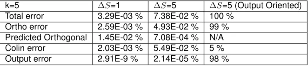
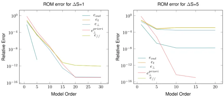
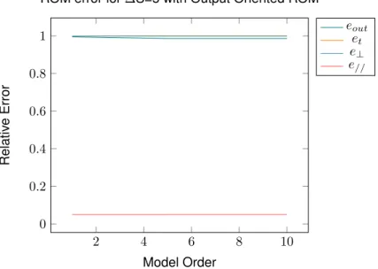
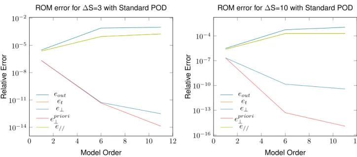
The magnitude of the eigenvalues ​​does not decrease as fast as the eigenvalues ​​of the dynamic problems. It therefore seems futile to use these methods as a way to reduce the error in the Galerkin projection. In the case of the output-oriented ROM, this only affects the SVD calculation, but it does so in a severe way, destroying the performance of the method.

Table 3.8 presents the coefficients of the article and the version we used as a benchmark. As can be seen, the ROM solving time dominates the POD calculation time. We hypothesized that this is due to the limited number of snapshots used and the non-linear nature of the problem, which naturally means a higher workload for the CPU.

In fact, Galerkin's ROM using the "fsolve" function can provide a solution in almost one-tenth the time of the least-mean-squares ROM.

CFD Analysis and Reduction

Introduction

Choice of Solver

The domain decomposition itself starts by a call from the constructor of the class "CDriver" to the constructor of the. The terms of the PDE to be solved (fluxes and sources) are calculated by calls to the . CSolver" class and the rest of the corresponding ODE is calculated by the "CIintegration" class.

The iterations themselves (and thus the solution of the model itself) are performed by calling the "Iterate" method of the "CItration" class ("CMeanFlowIteration" for the Navier Stokes equations), which itself will call a method in "CIintegration" class ("SingleGrid Integration" if we don't use multi-grid methods). The complexity of the code is immediately apparent, and were we to try to implement either manual zone selection for domain decomposition or the use of reduced-order models, it would likely take far more time than what is available for the conclusion of a master's thesis. To implement the desired domain decomposition, we would need to change CPhysicalGeometry and how it handles ParMETIS, and make sure that the rest of the.

Then we need to make sure that CIteration, the class responsible for performing an iteration of the solver, reduces the reduced residual. We expect that this will dramatically reduce the time required to test the various methods we wish to test. In the rest of the chapter, we will test the available FreeFem++ models for compressible Euler and Table 4.1: Solver decision matrix.

We will then reduce the patterns present in these scripts using LMSQ reduction and Galerkin projection and conclude on the performance of the MOR techniques.

Incompressible Navier Stokes

• Verification
• Validation
• Reduction

For this reason, for the validation of this script, we have decided to compare the results of the HMD in the script directly with the results in [112]. We will determine the relative deviation of the data obtained through the script compared to the references [112] and [113]. We will now attempt to perform the MOR of the Lid-Driven Cavity problem previously used as a benchmark.

The original author of the script [109] claims to reduce the lid-driven cavity by performing the POD of snapshots taken forRe and 151. Still, we hope that with up to 200 subdivisions we will be able to capture the efficiency trend in ROM 'one. As discussed in previous chapters, for the POD we compute the SVD of the snapshot matrix and take the first four left eigenvectors.

This is because in the original script the average of the solution samples was subtracted from the snapshot matrix. The final observation is that the ROM response of the original script for Re = 101 has a non-negligible error, as shown in Figure 4.12. This can be made possible by using tensors instead of matrices to discretize the PDE in 4.3.

The performance of the BFGS algorithm (and most optimization algorithms for that matter) depends heavily on the starting point given to the optimizer.

Compressible Euler

• Verification
• Validation
• Reduction

To validate this script, we will implement the RAE-2822 airfoil test case as specified in the AGARD report in [80]. For the airfoil shape, we used a spline interpolation of the design points (not experimentally measured) contained in the report and chose a unit chord (instead of the 0.61 m given in the report). Care was taken to match the non-dimensional length used by the solver with the airfoil length used for the RAE-2822 grid.

For the reduction tests, we will perform the same kind of sweep and scalability tests that were done for the NSI comparisons by changing the angle of attack of the airfoils. This means that for the supersonic model we will use the conditions and mesh element sizes specified in the script. For the RAE-2822 model, the geometry and conditions are the same as in the validation case, but the field boundary is closer than before.

For the Rae-2822 case, we give the Cauchy residual CL and CD for the scalability tests in Table 4.9. The results for the sweep tests and the resulting aerodynamic coefficients can be seen in Figures 4.70 to 4.73. As can be seen, we obtain errors below 1% for most of the sweep for the RAE-2822 airfoil with almost perfect fit of the aerodynamic coefficients.

This is exemplified in Figure 4.74, where it is shown that throughout the sweep the Cauchy residual in pressure for the ROM is less than that of the HDM.

Conclusions

Achievements

Overall, we have demonstrated that using the Proper Orthogonal Decomposition with either the Galerkin projection or the Least Mean Squares Reduction methods can be used to create reduced-order models that are significantly faster to compute (>2×faster ) while keeping errors below 10 % in most. cases, and without requiring many previously calculated samples (in the CFD analysis and reduction, the largest number of samples taken was 5). This property appears to be lost through time discretization error when using time marching methods, but the errors remain low (<1%) near the points where the samples were taken. We also note that so far no loss of stability has been observed using reduced order modeling, even when simulating the compressible Euler equations, where no physical viscosity is present.

These methods exhibit larger deviations when more than one parameter is varied or when strong point singularities are present.

Future Work

Bibliography

Goal-directed, model-constrained optimization for reduction of large-scale systems. Journal of Computational Physics. A low-cost, purposeful 'compact proper orthogonal decomposition' basis for model reduction of static systems. Reduced order modeling method via proper orthogonal decomposition for flow around an oscillating cylinder.

A training set and multi-baseline generation approach for parametrized model reduction based on adaptive grids in parameter space. A flexible and efficient greedy procedure for optimal training of reduced-order parametric models.