Multi-Stage Model Predictive Control for Trajectory Tracking problem on a real autonomous car

After describing and verifying the physical phenomena acting on a vehicle, the concept of the Model Predictive Controller (MPC) is described and how it can be applied to this trajectory following problem. With that, the implementation details will be scrutinized to deal with this strategy.

List of Tables

List of Algorithms

Acronyms

Introduction

• Autonomous vehicles
• Car Transformation
• Control Strategies
• Historical Review
• Model Predictive Control
• Vehicle Control
• Vehicle Parameterization
• Thesis Contributions
• Thesis Outline

Those modifications are like putting sensors on the vehicle like cameras, light detection and ranging (LIDAR) or sonars. The interactions between these competencies and the vehicle's interactions with the environment largely depend on the driving scenario (highway, urban driving, parking, racing, etc.) [21].

Vehicle Dynamics

• Vehicle Kinematics
• Bicycle Model
• Tire Model
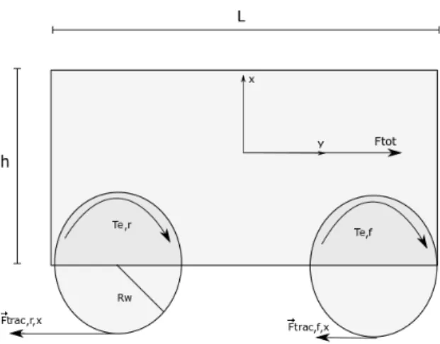
• Actuating Forces
• Forces caused by turning
• Acceleration forces
• Dissipative forces
• Total force actuating on the vehicle

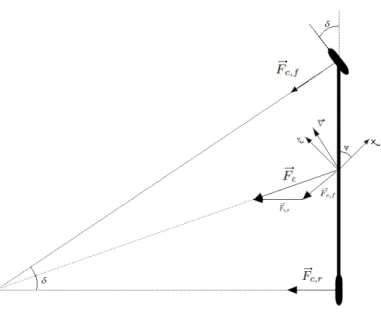
It is good to notice that the vehicle is running on a straight track (α= 0), the lateral force caused by the tire is also zero. During turning, while the steering angle is non-zero, a lateral force exerted on the vehicle by the curve pushes the car into the center of the curved circle. A similar behavior occurs at the rear of the vehicle, but in this situation a lateral force.

The acceleration of the vehicle exists because of the torque produced by the engine, applied to the rear wheels. Although the force produced by the vehicle can be considered as the total force applied to the vehicle, one must consider the dissipative ones. It is possible to conclude that the total force applied to the vehicle is the force produced, reduced by the dissipative effects, as shown in the following equation.

Vehicle model simulation

Car Parameters

All other necessary constants, such as vehicle inertia, can be derived using the equations presented in Chapter 2 and in [39].

Simulations

• Motion analysis
• A Steering angle analysis
• B Acceleration analysis
• Actuating forces analysis
• A Dissipative Forces (fig. 3.6)
• C ”Rotational” Force
• D Force Produced

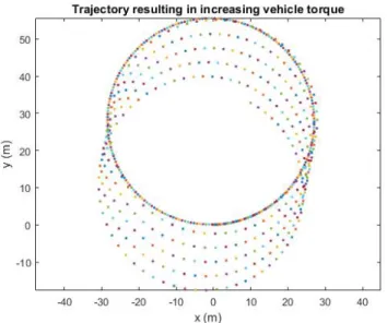
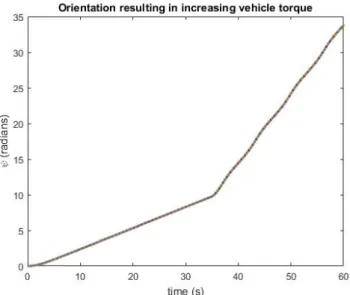
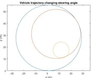
After analyzing the steering angle, the second control parameter of the vehicle is the engine torque, which is responsible for the acceleration of the vehicle. This situation happens indefinitely, causing the vehicle to fluctuate in speed and also in orientation, as can be seen in Figure 3.16. During cornering, one of the main actuation forces on the vehicle is centripetal.

This happens mainly due to the fact that with a smaller steering angle the vehicle's velocity is lower, which causes a lower centripetal force. Due to the torque applied to the vehicle wheels, tire's lateral force, centripetal and "rotation". This happens due to the fact that the vehicle's speed is lower, as the radius of curvature is also lower.

Model Predictive Control

Multi-Stage Non-linear MPC

• Robust Multi-stage Non-linear MPC
• Robust horizon

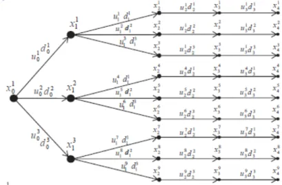
This technique is applied again to each of the generated new states until the forecast horizon is reached. Since more details will be given later, the vehicle control input signal briefly consists of two variables: the engine torque and the steering angle. Each uncertainty value taken at each branch of the MPC tree is predefined.

With this, the tree structure will increase its dimension, which can be problematic when expanding each node, as more computation time will be taken to compute the control signal with this new feature. The results obtained in chapter 2 and appendix A will be evaluated with relevant simulations based on realistic events that can happen in a real vehicle. The results obtained will be examined to prevent any possible unexpected behavior on the real system.

MPC implementation

• State definition
• Trajectory definition
• MPC structure

One major drawback of this approach to dealing with uncertainty is that complexity increases with the power of Np, the forecast horizon. One solution proposed in [40] is to, starting at a certain point, only extend the state itself with one type of uncertainty, as figure 4.1 shows, which the next state can also follow this approach. However, since we are dealing with a real-time autonomous vehicle, this approach is not plausible.

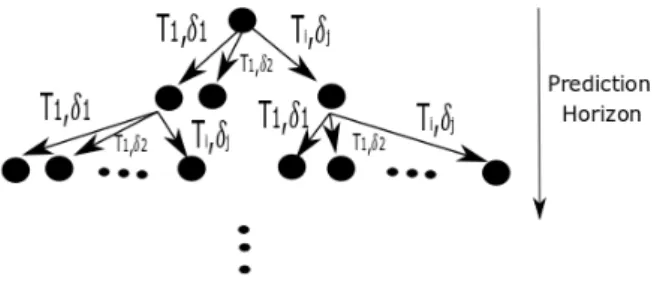
In each of these states, the cost associated with the value function and a new set of states were calculated. The multistage MPC pseudocode is presented here to facilitate understanding in the implemented algorithm. To evaluate this implementation, a set of tests was created to understand the impact of the cost function parameters and the control horizon it would take on trajectory tracking for different trajectories.

Simulations

• Trajectories
• A Straight trajectories
• B Pseudo Oval Trajectory
• C Eight-like Trajectory
• Cost Analysis
• Prediction horizon and computational time
• Sampling time
• Trajectory tracking at constant velocity

A larger value of Q3,3 would lead to a more rigid result on the vehicle's orientation regarding the trajectory. Although it would be expected that increasing the value would lead to a stricter following of the reference, one can notice that this is not the fact. In this one, where two full rotations were made, passing the critical situation of the transition limit on the vehicle's orientation, as it is defined between [0,2π[ the results obtained were satisfactory.

To solve this situation, it was proposed that instead of having control over the speed and steering angle of the vehicle, only have control over the steering angle. Finally, it is also possible to reduce the number of states (whether or not to increase the number of possible values ​​for the steering angle) and have a larger prediction horizon without increasing the execution time of the MPC. To verify the increase in cornering smoothness, one can compare the vehicle's orientation variation with.

Conclusion

This was intended to serve as a controller device to simulate vehicle behavior for several different trajectories. To perform this verification, a large set of tests was made in Chapter 3 with all the related situations that could exist considered. Then, implementation details were investigated to validate the vehicle dynamics controller approach as an MPC device.

Knowing that a trajectory tracking system must respond quickly, it is necessary to have a short sampling time to be able to process new (and possibly unexpected) information, not only trajectory information, but also measurement information. Even if all the desired features for trajectory tracking on a real vehicle were implemented, considerable work is still needed to have a fully functional algorithm. This work may start with the implementation of the same algorithm described here to perform the trajectory tracking tests on the Fiat Seicento Elettra.

Bibliography

Ackermann, “Robust car steering by yaw rate control,” in 29th IEEE Conference on Decision and Control, Dec. 1990, pp. Goodwin, "Adaptive trajectory tracking control of skid-steered mobile robots," inRobotics and Automation, 2007 IEEE International Conference on. Luo, “Experimental local model predictive control: Trajectory tracking and cost function tuning for wmr reactive navigation,” IFAC Proceedings Volumes , vol.

Wellstead, “Estimation of Vehicle Lateral Velocity,” in Proceedings of the 1996 IEEE International Conference on Control Applications IEEE International Conference on Control Applications Held in conjunction with IEEE International Symposium on Intelligent Combat, Sep 1996, pp. Gerdes, “Estimation of vehicle roll and road bank angle,” in Proceedings of the 2004 American Control Conference, vol. Sienel, “Estimation of tire torsional stiffness and its application to active car steering,” in Proceedings of the 36th IEEE Conference on Decision and Control, vol.

Model Predictive Control Theory

Linear MPC

The MPC, also known as Reeding Horizon Control (RHC), Model Based Predictive Control (MBPC) or Moving Horizon Control (MHC) is a control technique where the current control action taken at the current step is given by a finite horizon open loop optimal control problem and next action, is chosen as a result of the minimization of a value function, expressed as the one given by equations (A.2), with as initial state the current state of the plant [12]. This cost function can be divided into two main components: The first term corresponding to energy of the state and the second one to the control signal, where the current system state isxi denotes the current control signal. The open-loop optimal control problem, shown in equations (A.3), is based on the minimization of the cost function like the one presented in (A.2).

These constraints are made to prevent the state variables and the control signal from exceeding certain thresholds, as in (A.3b) and (A.3c), where lower and upper bounds are specified. Also the linear discrete time system expressed in (A.3d) which defines the dynamics of the systems and where xandu are defined in a set of admissible states that act as constraints in the minimization problem defined in its feasible subset. After the minimization process along the horizon, the first control signal of the corresponding optimal sequence, u∗, is applied to the system.

Non-linear MPC

After this process, the state is updated and this minimization is repeated for the new system state. The cost function is now defined as in equation (A.5), with a slight change compared to (A.2) - the terminal constraintF(xNp). This functional can also be rewritten as equation (A.6) for the purpose of notational simplification, since it will be used repeatedly.

Stability

To extrapolate these obtained results from continuous time to discrete time, since the implementation is in discrete time, one can consider discretization methods that do not contradict the assumptions implicit here. Let Xi, for any integer, be the set of possible states, by an admissible set of checks for Xf. It is necessary to determine a control set for x˙ and thus an upper bound for Vn(( ˙x)). To obtain a feasible check for this minimization problem, it is necessary to add an additional check element, kf(N;x), tou∗(x)en as the check law stated in (A.9) is applied, the following properties are true. A.17) The cost associated with this artifact is thus given by equation (A.17) and provides an upper bound for Vn(˙x), which satisfies.

So, if the following four conditions are met, the closed-loop asymptotic (exponential) stability is ensured. This means that the condition constraint is satisfied in Xf (condition 1), the control condition is satisfied in Xf. condition 2), Xf is positively invariant under the control law kf (condition 3), and that F is a local Lyapunov function (condition 4).

Discretization Methods

• Euler melhod
• Taylor expansion
• Automatic differentiation
• Runge Kunta and other methods
• Rounding errors and numerical stability

Starting from the initial condition, the evolution of the system is shown with a step size (h) indicating the rate of discretization. A function can also be represented by an infinite sum of terms, given by the derivative functions. The Taylor expansion expresses the mathematical model between this idea, presented in equation (B.3). B.3) In the above expression you can see that high order terms can be ignored.

This method uses the assumption that a function can be broken down into a set of simpler functions, represented by the four basic mathematical operations, addition, subtraction, division and multiplication, where the derivatives are familiar and simpler, and also functions such as exponential, trigonometric and logarithmic . Although the majority of systems can be described by the methods mentioned above, Runge-Kunta methods and others can be used to accomplish this task. If, at each iteration of the Euler method, a round-off error occurs at (not a very likely situation, since the error should occur in the same direction, increment or decrement), the total round-off error in steps will be of the order of magnitude.