The second fact has led researchers to incorporate heterogeneity in price stability into the standard models to study its positive implications. In contrast, the weights on the sectoral output gap are the same across sectors, meaning they should move similarly in response to shocks. The increase in taxation is proportional to the degree of price stability in the sector.
The optimal paths for inflation and production remain qualitatively the same as in the sector-specific tax case. Since the social planner will face the same incentives at each date, the solution would involve deviating from the commitment to a lower level of inflation in the first period and committing to low inflation in the future. Welfare in the case of homogeneous price stability depends only on squared deviations of inflation and the output gap.4 This result rationalizes the usual loss function assumed in the monetary policy evaluation literature.
The second rule implies that in the optimal equilibrium the price level must follow a random step.
Approximate Model
The first implicit targeting rule takes the form of flexible inflation targeting, similar to the case of flat taxation as in Woodford (2003). In this section, we describe a log-linearized system that characterizes a heterogeneous price stickiness economy and derive its loss function. This sectoral Phillips curve is similar to the case of homogeneous price stickiness in the sense that contemporaneous inflation depends on output and expected future inflation.
If the elasticity of substitution between different sectors is high (η−1 close to zero), a higher aggregate output leads to higher sectoral inflation. The target tax rate τ∗k,t is a linear function of aggregate government spending, sectoral shocks and aggregate productivity, as well as average disturbances in the labor market and other parameters of the economy (defined in Appendix F). It is a linear function of assumed stochastic disturbances in the labor market and other parameters of the economy.
The government's solvency measured by its real value of its liabilities (ie: ˆb∗t−1−πt) depends negatively on sectoral taxation and aggregate output (tax base).
Welfare
This loss function differs from the function derived without price heterogeneity in two ways. First, square deviations from sectoral inflation appear in the loss function instead of aggregate inflation. The greater the price stability in a given sector, the greater the relative importance of inflation in that sector in the loss function.
Unlike the homogeneous case, the convexity of the loss function as well as the different weights between sectors imply that, given a shock, there is an optimal sectoral inflation spread. Second, the usual negative effect of total output gap volatility on welfare gives room to the sum of sectoral output gaps. Therefore, the same cross-sector weight and the convexity of the loss function will imply strong shifts of sectoral output gaps under optimal policy.
In this section we find the approximate solution to the Ramsey problem, described in section 2.3.
Policy Problem Solution
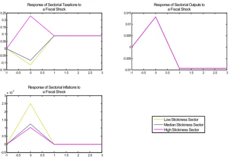
Fiscal Shocks
By keeping the median stickiness of the economy at the same level and making price stickiness more spread out, it is possible to obtain a positive initial response. Heterogeneity in price persistence does not change the optimal response of aggregate output gap, as seen in the first panel on the right; only the long-run levels differ slightly due to different levels of long-run aggregate taxes. Intuitively, the optimal policy takes into account the inflationary effects of higher taxes in sectors with lower stickiness.
Therefore, the tax adjusts only moderately, as expected in light of our discussion of the loss function. 6 We consider three cases: a homogeneous economy, where the degree of price stability is set to be 0.5 for each of its three sectors; a low-variance heterogeneous case, where sectors present a nominal adjustment probability in each period of .2, .5, and .8; and a high variance case, with probabilities .1, .5, and .9. Risk aversion is set to 2, the inverse of the Frisch elasticity is set to 0.47, the within-sector elasticity of substitution is 10; cross-sectional elasticity of substitution is 4.5; government consumption is set at 22% of GDP; with a real surplus of 2%, and an annual level of debt over GDP of 50%.
Discount factor is .99, lambda is set to .98 and 1.05 is the steady level of gross wage markup.
Cost-push shocks
Welfare Analysis
As can be seen, the impact on losses of consumption equivalents can be relevant under stable conditions: in the case of a low dispersion of sectoral price stability, this leads to losses of 0.022% to 0.057%, depending on the parameters used. In the case of high dispersion, this leads to higher losses, ranging from 0.201% to 0.489%, depending on the calibration. Given the average level of household spending on the US economy in 2006, these welfare losses imply that in the first case, every US household would consider making one annual payment of $10 to $27 to ensure a fully informed policymaker.
In an economy with wide dispersion in price stability, this amount would be from US$99 to US$237, respectively. We do this to distinguish which results come from the heterogeneous stickiness and which come from the heterogeneous taxation assumption.
Response to shocks
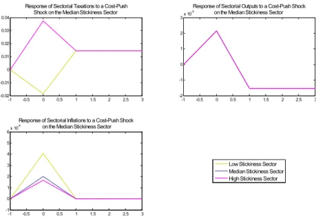
The effects of sectoral cost pressure on aggregate variables lead to similar insights as those in the case of a fiscal shock.9 However, uniform taxes significantly change the dynamics of sectoral variables. As can be seen in Figure 7, the sector affected by the cost shock (i.e. the sector with no change in the median) behaves normally: inflation rises while the output gap narrows. To offset these effects, the optimal policy lowers taxation, leading to higher levels of public debt.
In the absence of a sectoral instrument, this tax cut is applied to all sectors, leading to deflation in those sectors not affected by the shock. The output gaps in these sectors are widening not only due to lower taxes, but also due to the substitution effects of price increases in the sector affected by the shock. In particular, taxation under an optimal policy follows a staggering adjustment to a positive level in the subsequent dates.
Welfare Analysis
In particular, taxation under optimal policy follows a surprising adjustment to a positive level in the subsequent dates. sectoral inflation dispersion in response to shocks. Second, welfare also depends on the squared deviation of each sectoral output gap with the same weight. This suggests that sectoral output gap misalignments should be avoided under optimal policy paths and that there is a role for sector-specific policy instruments.
We show that the optimal targeting rules and the responses of inflation, the output gap, and public debt to shocks are different in the presence of different levels of price invariance. In addition to theoretical considerations, realistic models for optimal fiscal and monetary policy should consider not only aggregate but also sectoral data for calibration. We believe that such a framework would enable a quantitative evaluation of the welfare consequences of heterogeneity and sector-specific policy instruments.
Price determination in the euro area and the United States: some facts from individual consumer price data. Journal of Economic Perspective. Comparing Shocks and Frictions in US and Euro Area Business Cycles: A Bayesian DSGE Approach.” Journal of Applied Econometrics. Solving dynamic general equilibrium models using a second-order approach to the policy function.” Journal of Economic Dynamics and Control.
In this case, the distortionary tax rates in the steady state are the same in all sectors, i.e. When considering the always possible normalization Y¯ = 1, the only constraint is that the level of consumption relative to GDP cannot be too high for tax rates to be positive. In order to impose constant bounds X0 = ¯X, we consider additional constraints, such as first-order conditions for the int=t0 problem, equivalent to first-order conditions for the generic >0.
To complete the proof, we need to show that the first-order conditions for the indicated steady state are satisfied for time-invariant Lagrange multipliers. After taking FOCs from the maximization problem, it is possible to show that the system of steady state variables and time invariant multipliers is just identified.
Second Order Approximation of Utility Function
Using a second-order Taylor expansion on the law of motion for the sectoral distribution of prices given by. Here we consider the sectoral distribution of prices in the distant past as a “policy-independent term”.
Second Order Approximation to AS Equation
Considering the expression for Kk,t, define Πk,t,s =Pk,s/Pk,t, where s ≥ t is some date in the future and Pk,t is the aggregate price level in the sector in period t. Taking the expression in the text for Fk,t given by (24), we define the net revenue factor as Γk,t≡1−τk,t and use the Taylor expansion of the second order:.
Second Order Approximation to the Budget Constraint
Aggregate and Sectorial Output Relation
Matrix Notation
Elimination of Linear Terms
Definitions of Qxx and Qξ in terms of economy parameters defined in the Technical Appendix. As in Benigno and Woodford (2003) and Ferrer (2005), references to sectoral tax rates have been removed. Only references to sectoral measures of inflation, sectoral and aggregate output remain, meaning (93) that they can be further simplified by removing references to tax rates and by separating terms relating to sectoral and aggregate output from references to sectoral inflation .
Assuming that wage premiums are stable and that marginal cost premiums are the same in all sectors (¯µwk = ¯µw and θk=θ), q-coefficients are all independent of k. Yˆk,t∗ =λ−yk1[(qyG+qykG) ˆGt+qykakˆak,t+qykµkµˆk,t] (107) allk, and, more importantly,λyk andλk,π give the weight of each of these terms in the welfare based criteria. In addition to the full definition of such terms, the Technical Appendix covers the conditions for concavity.
The coefficient definitions of the optimal targeting rules are given in terms of the parameter in the model presented in Section 2 as .
Definition of Target Variables
Aggregate supply and cost-push disturbance term
Averaging across sectors allows us to determine the general aggregate first-order approximation for the AS equation in (33), similar to Carvalho (2006).
Budget Constraint and fiscal disturbance term
Aggregate and Sectorial Output Relation