Os resultados analíticos mostram que em algumas situações ter uma asa batendo tem melhor desempenho. Palavras-chave: vibração de asa, comparação, teoria dos elementos da pá, potência, aerodinâmica instável.
List of Tables
Nomenclature
Acronyms
Introduction
- Motivation
- Topic Overview
- Configurations Comparison
- Flapping Flight Models
- CFD Analysis of Flapping Flight
- Objectives
- Thesis Outline
However, the subject of forward flight remains largely unexplored due to the difficulty of the analysis and the wide variety of factors that play a role in the flight of a flapping wing vehicle. Even if all the mentioned studies apply to the case of hovering vehicles and animals, the same search focused on a BET model for forward flapping flight returns no results.
Background
Power Consumption
- Fixed Wing
- Rotary Wing
- Flapping Wing
At this point, the parameter σ is introduced, which is the solidity of the rotor, defined as the ratio between the total surface of the blades and that of a filled circle with the same radius. The only thing missing is the initial value, which, in most cases, can be assumed to be equal to the hoverλ=pC value.
Blade Element Theory
- Forward Flight
While the state of flight is the mode of flight most commonly studied with this method, it is also possible to model forward flight, although this means adding several layers of complexity to the problem. Two very important concepts needed now are the blade azimuth angle and also the angle of incidence, both shown in Figure 2.2.
![Figure 2.2: Side and top view of the blade, showing the flapping angle γ and the azimuth angle ψ, respectively, as well as the relevant velocity components (adapted from [11] and [12]).](https://thumb-eu.123doks.com/thumbv2/123dok_br/19768636.0/33.892.124.770.314.530/figure-showing-flapping-azimuth-respectively-relevant-velocity-components.webp)
Hovering Flapping Wing Models
- Truong’s model
- Walker’s model
This is a really unstable part of the model because different values of G will appear as ω changes. The next step of the algorithm is to define the velocities needed for the calculations. According to the author, this is the element that effectively turns the model into an unstable one.
Force resulting from the circulation around the wing, while also taking into account the influence of the associated vortex via the Wagner function. Finally, the total instantaneous drag and lift forces are obtained by an integration along the wing span.
Preliminary Power Consumption Analysis
Fixed vs. Rotary
The first one is that the wingspan of the fixed wing is equal to the diameter of the rotary wing's rotor, or. Second, the weights of both configurations will be considered the same, meaning that the thrust of the rotary wing is equal to the lift of the aircraft. The expression also depends indirectly on the tip speed of the blades, Vtip, through the advance ratio.
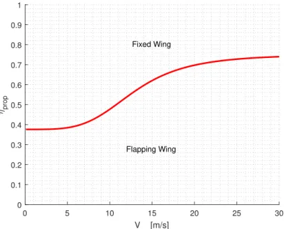
Since only the propeller efficiency varies along this line, this means that the portion of the graph above the curve represents areas of higher propeller efficiency, favoring the fixed-wing configuration. Increasing the aspect ratio of the fixed wing resulted, perhaps unsurprisingly, in a larger area where the fixed wing solution is better.

Fixed vs. Flapping
Now for the analysis of the results, to learn about the aerodynamic behavior of the configurations and to conclude which are the aspects that most influence their performance: starting with the angle of impact, shown in Figure 3.4(a), it is clearly this is one of the factors that most determines whether a flap configuration is more efficient than its fixed-wing counterpart. It can also be seen that an increase in flap angle means a worse overall performance for the flap configuration, as the curve shifts downward (reducing the area for which the flap is preferential). This is due to the fact that a larger angle of attack means that a higher percentage of the total lift generated will not be vertical.
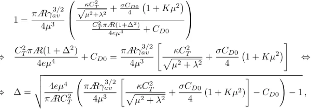
When talking about the speeds in the intermediate range, increasing the aspect ratio benefits the fixed wing and increasing CD0 benefits the flapping wing, but for both small and high speed values these parameters become irrelevant as the curves all collapse into the same line. It can be observed that the case of ∆ = 0 is the ideal scenario where the Oswald coefficient would not change for the flapping case, meaning there would be no loss of efficiency due to the movement of the wings.
Rotary vs. Flapping
First, for very high advance ratios (since in this case Vtip = 56.14 m/s, this means forward speed of about 18 m/s) there is no case where the flapping wing is more efficient than the rotary wing. The aspect ratio of the flapping wing, analyzed in Figure 3.6(b), plays a very important role in its performance as small variations to this value mean completely different results, something that can be concluded by looking at some specific cases to look at: for anA= 2, after µ= 0.27(V∞≈ 15 m/s), there is absolutely no case where the flapping wing is more efficient. The flap angle, seen in Figure 3.6(a) also shows some influence on the performance of the flapping wing, as it can be observed that its increase reflects itself on a decrease of the favorable area of the flapping wing.
This is consistent with what one would predict, since the same increase in flap angle does not have an equal impact on the slope of the lift vector for small angles (see lines defined at γ=0°, the fixed airfoil, and γ= 15 °, where the difference is barely noticeable), as when the angles are already close to vertical (see lines defined at γ=75° and γ=90°, where the same increase of 15° resulted in a much smaller area where flapping is favorable ). The profile drag coefficient, visible in Figure 3.6(c), shows a relatively small effect on power consumption; a smaller value of CD0 appears to be beneficial for the flapping wing option, but for higher speeds this value becomes irrelevant as all the curves collapse to the same.
Development of an UBET Model for Flapping Wing Forward Flight
Hovering Models
- Truong’s Hovering Model
- Walker’s Hovering Model
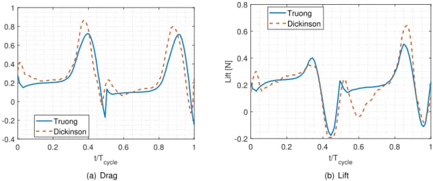
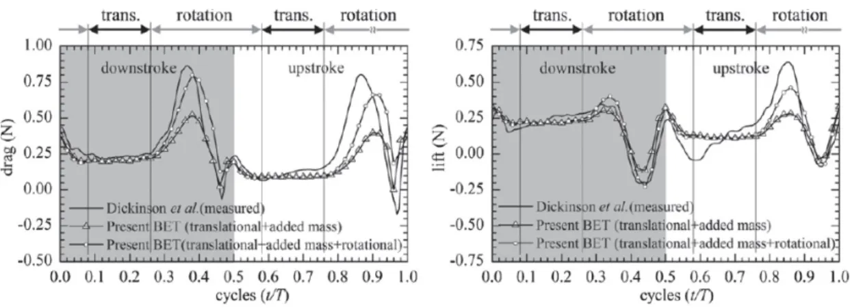
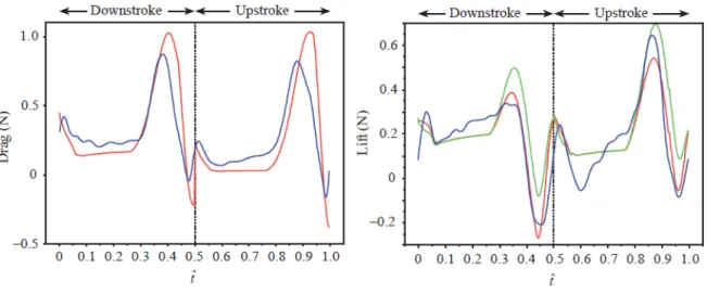
Especially at the points of stroke return (meaning at the middle and end of the cycle) the rotating wing generates the extra force it needs through the predicted unconventional methods, in this case from pushing the air around it (added mass force) and taking advantage of the circulation established by the wing's own previous motion (rotational force). Now comparing the total lift and drag values with those measured by Dickinson [5], as seen in Figure 4.4, it becomes clear that the model provides a good approximation of the forces generated by the wing. Instead of the three components predicted by the first model (translational, rotational and added mass), here it is assumed that there are only two (rotational and added mass).
To complete the process, you must again turn to integration along the wingspan, and the last step is to plot the results. Regarding the output of the MATLAB routine, first is the plot of the force components, both for lift (Figure 4.5) and drag (Figure 4.6).
![Figure 4.1: Scheme of the experimental setup used by Dickinson et al. [5].](https://thumb-eu.123doks.com/thumbv2/123dok_br/19768636.0/60.892.300.590.226.490/figure-scheme-experimental-setup-used-dickinson-et-al.webp)
Adaptation of the Hovering Models to the Forward Flight case
- Modified Truong Model for Forward Flight
- Modified Walker model for Forward Flight
- Joint Model
This is the justification of the approach adopted in this work to model the flapping flight, which briefly corresponds to a change in the reference axis and a different definition of the velocities relative to the wing. After the measurements, Leishman developed the following equations for the lift, drag and moment coefficients of the NACA 0012 airfoil. Since Walker views the wing angles in a different way, this difference is reflected in the determination of speeds.
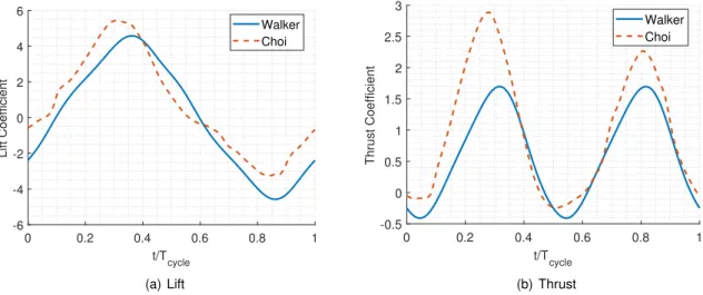
This is a better approximation than Truong's because it takes the rotation of the wing into account. In contrast, Walker's model shows surprising precision in terms of thrust estimation.
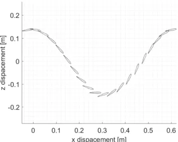
![Figure 4.8: 2D trajectory of a flapping wing in forward flight, along with its wake (adapted from [19]).](https://thumb-eu.123doks.com/thumbv2/123dok_br/19768636.0/66.892.129.758.240.365/figure-trajectory-flapping-wing-forward-flight-wake-adapted.webp)
Tool Development
- Absolute Analysis
- Variable Dependant Analysis
- Steady State Analysis
The user then has the option to change any parameter that is shown in the box marked with the number 4, which means there are a total of 9 variables that can be changed and. So the user can choose to study any of the nine parameters by leaving it as a variable, rather than adjusting its value. Still in box number 10, the user can also define the lower and upper limits of the variable.
Then, in the box marked with number 11, the user can select the values for each parameter, except for the values of the variable that was designated, in the same way as was done in the absolute analysis. After doing this, the user can press the Calculate button, which prompts the tool to start the calculations.

Refined Power Consumption Analysis
Flapping Wing Performance Analysis
- Mass
- Aspect Ratio
- Maximum Flapping Angle
- Maximum Rotation Angle
- Average Pitch Angle
- Wing’s Rotation Center
- Wingspan
- Flapping Frequency
- Forward Speed
- Steady State Analysis
The results are presented in Figure 5.4 and it can be seen that the aspect ratio plays a key role in terms of flapping performance. The flutter amplitude, represented by the letter γmax, is probably a very important factor in the overall performance of the configuration. Finally, looking at the power curve, we can conclude that this change, as expected, had an undeniable effect on the vehicle's energy consumption.
The center of rotation of the wing should in principle influence the loads on the wing in a relevant way. The combination of higher speeds and forces also means, due to the way power consumption is defined, that the power intake of the vehicle will increase dramatically with the increase in flap frequency.
Configuration Comparison
- Fixed vs. Flapping Wing
- Rotary vs. Flapping Wing
What can be observed is that, through this rudimentary optimization, energy consumption values similar in magnitude to those of the fixed arm were obtained. The results in terms of overall optimization were, however, not as pronounced as desired, with the most efficient flapper wing still consuming 104%. However, what can be gleaned from this study is that for roughly the same specs, the fixed arm has the edge in terms of power consumption.
Optimizing for the lowest possible power consumption and using steady state analysis resulted in the values shown in Table 5.2. There is still no point where the flapping arm outperforms the rotating arm, but the second case shows an energy consumption only 22% higher than that of a rotating arm carrying the same load and moving at the same speed.

Conclusions
Achievements
The model development also led to the creation of an instrument that can be easily used by anyone trying to study flapping wings. Being user-friendly and working quickly, the tool opens up several possibilities in terms of optimization studies and preliminary wing design. This is the legacy of this work in terms of an interactive, useful, physical product that anyone will be able to use in the future.
Finally, on the topic of optimizing the flapping wing, the tool was put to the test and a simple optimization was performed. The values resulting from the optimization could then be collected into two perfect flapping wing designs, and these optimized wings were then compared to the other configurations, finally providing the answer to the question "is a flapping wing really worth it?" ", which is, in short and in the right circumstances, likely.
Future Work
Bibliography
![Figure 2.1: Top and side view, respectively, of the reference scheme and wing environment used throughout this work (adapted from [11]).](https://thumb-eu.123doks.com/thumbv2/123dok_br/19768636.0/32.892.121.767.597.769/figure-view-respectively-reference-scheme-wing-environment-adapted.webp)
![Figure 2.4: Time history of the traslational (green) and rotational (purple) velocities of the wing [5].](https://thumb-eu.123doks.com/thumbv2/123dok_br/19768636.0/35.892.182.701.715.899/figure-time-history-traslational-green-rotational-purple-velocities.webp)
![Figure 2.7: Scheme of the parameters used by Walker in his analysis (adapted from [7]).](https://thumb-eu.123doks.com/thumbv2/123dok_br/19768636.0/41.892.225.647.118.419/figure-2-scheme-parameters-used-walker-analysis-adapted.webp)