O desenvolvimento de controladores de piloto automático de mísseis foi uma tarefa complexa, dado o envelope de voo estendido e sua dinâmica não linear. Ainda não foi encontrada uma solução que possa sobressair tanto no desempenho nominal como na robustez face às incertezas.
Nomenclature
Acronyms
Introduction
- Motivation
- Topic Overview
- Objectives
- Thesis Outline
Some are basic RL concepts (cf. Section 3.1) and others are state-of-the-art RL algorithms and complementary features. After all this, the thesis will conclude with a brief summary of the most important achievements (see section 6.1) and some suggestions of directions for future research (see section 6.2).
Model
Modelled Dynamics
- Forces and Moments
- Flight Dynamics
- Longitudinal Approximation
- Reference Model
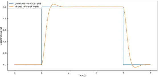
The dynamics of the rotation is characterized by equation (2.8), in which the dynamics of the body's velocity relative to the E-frameωE. Instead, the system will be required to follow shape reference signals, i.e., the output of the Reference Model.
Problem Formulation
The command reference signal (cf. section 4.3.1) is given as an input to the Reference Model, whose output, the formed reference signal, is the input of the agent. The former was defined as the L-2 norm of the four resting periods of the episode (cf.
Background
- Reinforcement Learning - Basic Concepts
- Trust Region Policy Optimization
- Reward Engineering
- Hindsight Experience Replay
- Prioritized Experience Replay
One way to branch all possible RL algorithms is whether or not the agent has access to the dynamics of the environment. Basically, the critic is an estimator of the rewards that the agent will collect when it performs a certain action. Sampling efficiency is a qualitative measure of the amount of observations an algorithm must collect from the environment to achieve a given goal.
Aˆπ,γ can be defined as the sum of the first elements1 of the sequence of states and actions that occurred (cf. Along, perhaps, with the exploration strategy, the reward function is one of the main features of the success of an RL algorithm. Schaul's hypothesis et al. is that significance should be defined in terms of Time Difference (TD) error (cf.
For high-reward agents (see section 3.3), the effects of this rarity are limited to an increase in convergence time.
Application of Reinforcement Learning to the Missile’s Flight
Reward Engineering
- Dense Exponential
- Dense Sum
- Sparse
- Dense Sum with SER
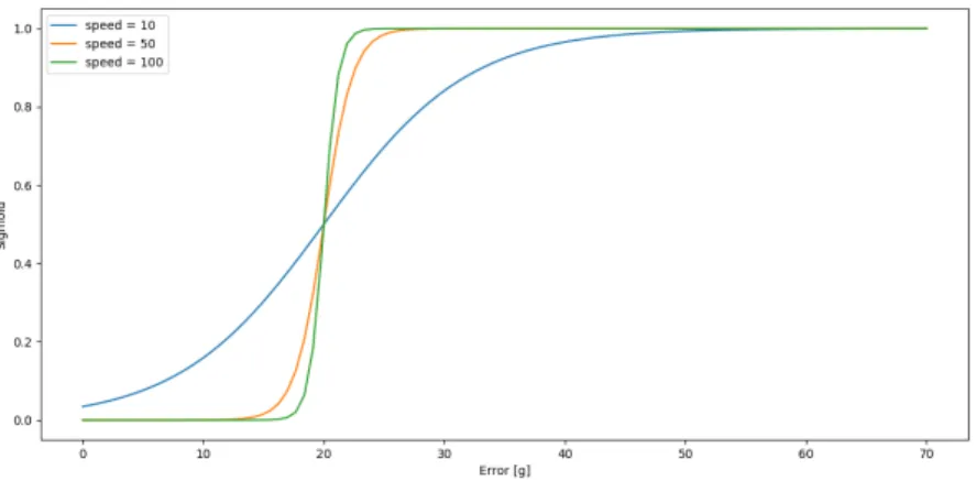
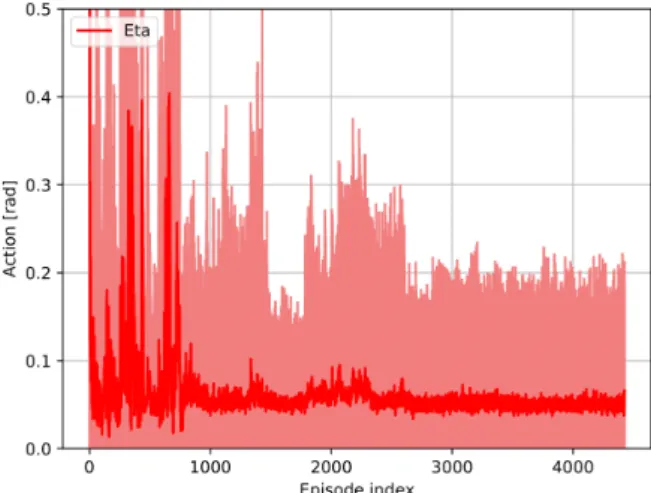
Moreover, a tendency was also observed for the performance objectives (see section 2.2) to be interrelated. Given a random initialization, the agent's first interactions with the environment typically result in a performance far from the target performance (see Figure 4.5), which iteratively moves closer to the goal. Despite the advantages mentioned in section 4.1.1, the exponential profile adds an additional level of complexity regarding the tuning process of the relative weights (wi, see Appendix A).
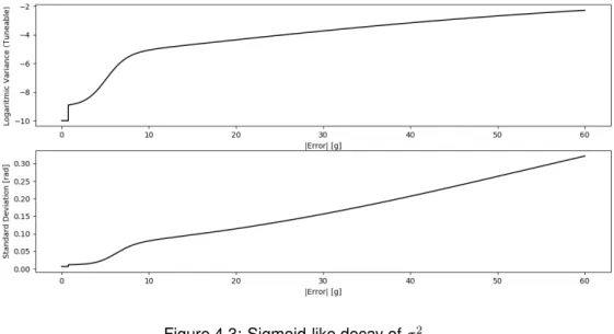
Finally, after reaching a suboptimal policy marked by an oscillating behavior of η in rest periods (cf. figure 4.1), f4 (cf. In fact, the problems associated with sparse CORF (cf. section 3.3) hold, also, for dense However, contrary to sparse rewards (see section 4.1.3), dense rewards are, alone, quite efficient in bringing the agent to the middle/near region and, therefore, the SER (see section 4.2.5) was implemented together with some CORFs from section 4.1.2 that had shown good train results, possibly with minor changes.
Considering the implementation of Section 4.1.2, configuration 1 modifies w3 and w4 (cf. Appendix A), decreasing them when |ez| grows so that the agent can be more agile in following the rise of the reference signal.
Algorithm
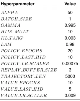
- Hyperparameters’ Configuration
- Modifications to original TRPO
- Hindsight Experience Replay
- Balanced Prioritized Experience Replay
- Scheduled Experience Replay
- Algorithm Description
The exploration strategy is the key to the sampling of new actions, included in step 1 of Algorithm 2 (cf. Section 4.2). In both strategies, apart from the step amplitudes, all the other original parameters (cf. section 2.1.4) of the reference signal are preserved. Having HER (cf. Section 4.2.3) and BPER (cf. Section 4.2.4) dependent on a condition - the SER condition - is hereby defined as Scheduled Experience Replay (SER).
The reward function that led to the target performance (cf. section 5.2) is nevertheless not sparse and could already reach the near region without HER. The actions are sampled according to the policy and the proposed exploration strategy (cf. section 4.2.2). With the above configuration, after it has been collected, the episode is over and therefore, if the SER condition (cf. section 4.2.5) holds, it is replenished according to HER (cf. section 4.2.3).
If the SER condition (cf. section 4.2.5) holds, the training dataset is sampled according to BPER (cf. section 4.2.4).
Methodology
- Command Reference Signal Generation
- Intermediate Tests
The criteria in table 4.6 have been established as a softer version of the requirements that define the target performance (cf. section 2.2). The definition of the criteria used to stop the train is the key to the success of the implementation, since, as chapter 5 shows, longer trains do not always mean a performance closer to the target. Furthermore, the need for table 4.6 to present higher thresholds than those of section 2.2 lies in the fact that the proposed exploration strategy (cf. section 4.2.2) never allows η's variance to be zero and therefore the test performance can be better than the one observed during training.
During training, Algorithm 2 is run with periodic interruptions where it is put on hold and an intermediate test is implemented to keep track of its progress. In all cases, after any test episode where, of course, there is no investigation (cf. Section 3.1), all the criteria defined in Section 2.2 are checked and the train terminated successfully if met and resumed otherwise.

Reproducibility Assessments
To highlight this issue, another nine training sessions were conducted with the same configuration, the results of which are discussed in Section 5.3, making a total of ten agents trained under the same conditions, with the following difference: when the best agent is trained found (cf. Section 5.2), both neural networks were randomly initialized, while the remaining nine agents were run loading the same initialization. Such a decision is made to consider only the effects of the factors that make up the design choice of an algorithm and, therefore, may be the subject of future research (see section 6.2). Furthermore, it has been observed that an agent whose training starts by restarting the training progress of another agent faces some instability in the first few episodes, which may cause its policy to deviate so much from that of the loading agent, that the loading benefits are void.
For this reason, in the reproducibility experiments, the configuration described in Section 4.2.1 was fully preserved, except for the value of KL T ARGET, which was set to 0.0001, which reduced the radius of the confidence region by a factor of 30, in a more cautious implementation experiment training.
Robustness Assessments
- Robustifying Trains
- Robustified Agent
In each case, four different values were tried for the limits of the range of possibilities (either maxor3σ), discarding the values for which the robust train had disintegrated after 2500 episodes. Introducing latency into the system means slowing down the effect of the action in the environment. This non-nominal environment therefore differs from the nominal environment in the presence of delay elements at the agent's output.
In this case, the M andh are estimated, the dynamics of which are significantly slower than those of the measured quantities under the considered flight conditions. The parameterization of the model's coefficients based on labeled data is not flawless and therefore it is important to know the agent's behavior in case of uncertainty. Aerodynamic coefficients, such as Cz and Cm, are of utmost importance because they are the basis for the dynamics of the longitudinal approach of the GSAM.
5To be precise, this interval only covers 99.73% of the possible values, but it is assumed to cover the entire spectrum of possible values.
Results and Discussion
- Expected Results
- Best Found Agent
- Training Evolution
- Test Performance
- Reproducibility Assessments
- Robustness Assessments
- Latency
- Estimation Uncertainty
- Parametric Uncertainty
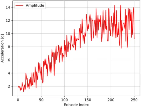
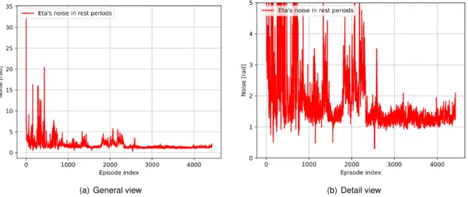
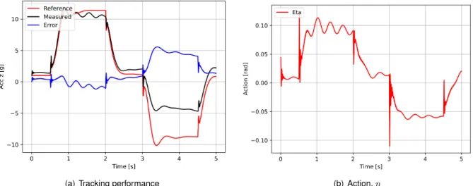
Since after this peak the magnitude η and the noise levels return to their previous stabilized (good) state and that there is a significant reduction in the tracking error between idle periods (cf. Fig. 5.4), it is reasonable to say that the adopted exploration strategy is properly oriented, which not enough to produce the desired policy divergence. As Figure 5.7 demonstrates, the agent is clearly able to control the measured acceleration and track the reference signal fed to it, meeting all the performance requirements specified in Section 2.2 (see Table 5.1). As Figure 5.9 shows, of the four different lmaxtried values, only 5 ms converged after 2500 episodes, which means that this was the only robust set that ran for a total of 5000 episodes, during which the best agent found was identified as with delay Robustified.
Compared to the nominal agent (see Figure B.1), the nominal performance of the latter (see Figure 5.10) is damaged, with a less stable action signal and poorer tracking performance. As Figure 5.11 shows, of the four different values of 3σ, only the 3% converged after 2500 episodes, meaning that it was the only reinforcing train that ran for a total of 5000 episodes, with the best agent found defined as the estimate. Uncertainty Robust agent. As Figure 5.13 shows, of the four different values of 3σ, only the 5% value converged after 2500 episodes, meaning that it was the only reinforcing train that ran for a total of 5000 episodes.
When compared to the nominal mean (cf. figure B.1), the latter's nominal detection performance is damaged, but the action signal is smoother (cf. figure 5.14).
Conclusions
Achievements
Future Work
In fact, the reward technique (see 1) is the most time-consuming phase of the entire process and avoiding it is a priority. To this end, approaches such as having sparse reward functions [28] or no reward functions at all [35] can be a source of inspiration. As section 4.1.3 showed, it is very likely that such a drastic simplification of the reward function will require deeper adjustments in the RL algorithm itself, even to the point where the algorithm to be implemented – in this case TRPO – is chosen due to the reward function and not the opposite.
However, since we know that DQN is not suitable for this task due to its discrete action space, it would be interesting to implement DDPG [6], DQN's continuous action space subalgorithm, with sparse reward and HER. This is especially important if the objectives become more complex when the implementation is extended to the full flight dynamics model as suggested earlier. As for 3, research could be done to find different techniques for the optimization phase of the neural network instead of ADAM, as they certainly have a strong impact on how the training of the parameters dictates the reproducibility of the results.
Finally, there is also room for improvement regarding the hyperparameterization (see 4), more specifically, to identify the optimality domains of each hyperparameter and the advantages of search algorithms such as Random Search [37] in the matching process.
Bibliography
Soft actor-critic: Out-of-policy maximum entropy deep reinforcement learning with a stochastic actor.35th International Conference on Machine Learning, ICML. Interpolated policy gradient: merging on-policy and off-policy gradient estimation for deep reinforcement learning.
Appendix A
Reward Engineering
Appendix B
Nominal Agent used in the Robustness Assessments
Appendix C
Reproducibility Assessment Experiments
Appendix D
Nominal and Robustified Agents’
Robustness Comparison