Furthermore, the experimental constraints on the radiation term are quite well known thanks to measurements of the cosmic microwave background (CMB) radiation. Similarly, we can comment on the value of the constant parameter (k=1 or 0) that allows us to distinguish between spatially closed (k= 1) and open (k= 0 or;1) universes: it is possible that the reduced cosmological curvature density k is very small, If the distribution of matter in the universe has some large-scale peculiarities (for example, a kind of "symmetry"), our solution to the above problem becomes phenomenologically important.
Most of this section is familiar and can be found in standard texts. In fact, the choice of sign (and name) turns out to be a historical error, since the last limits of the cosmological constant lead to a negative value for q (an accelerating expanding universe). The formulas giving the two periods !1;!2 in terms of the cosmological parameters k, and (org1;g2) involve elliptic integrals and will be given later.
This can be expressed in terms of a dimensionless quantity o (a particular value of ) or, more commonly, in terms of to =t(o). It can be thought of as giving a measure of the "total mass" of the universe. Since most experimental results are expressed in terms of dimensionless densities ;k;m;r, we express all other cosmological quantities of interest in terms of them. .
3 EXPERIMENTAL CONSTRAINTS
Experimental Constraints from High-redshift Supernovae and Cos- mic Microwave Background Anisotropies
One should not think that the value of can be arbitrarily large: we will see a little later (next subsection) that for experimental reasons it must also be bounded from above (condition ;< <. In light of the experimental results ( or small and ok compatible with zero), one may be tempted to make the simplifying hypothesis 1 = om+o, i.e. set both terms ok and ortho zero in the ratio 1 = m+k++r; note however that assuming the vanishing of k+rat all times (without assuming the vanishing of each term individually) is totally impossible, since these densities are not constant and it is easy to see, from the negation of these quantities, that such a relation can only hold for a single moment; it is clear that the radiative contribution, or, although small, is not strictly zero. Moreover, setting the constant k at zero is certainly compatible with the present experimental data, but one must be aware of the fact that the curvature density k is not a constant quantity and that setting it to zero at all times is an artificial simplification that was probably not justified when the universe was younger was not:::.
A Curious Coincidence
4 ANALYTIC BEHAVIOUR OF SOLUTIONS
Qualitative Behaviour of Solutions
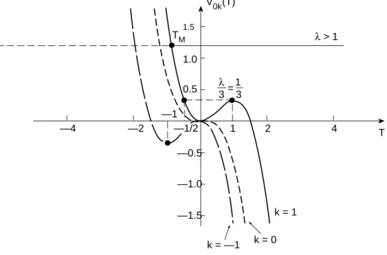
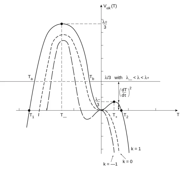
The only feature of casek= 1 is that there is an injection point (which comes from the existence of a positive maximum on the right-hand side for the V(T) curve): the expansion still speeds up, but there is a time for which the expansion rate vanishes.
The Elliptic Curve Associated with a Given Cosmology .1 General Features
- Neglecting Radiation : the Case = 0
- Not Neglecting Radiation : the Case 6 = 0
Finally, one must remember that the order of an elliptic function is at least two, and that the WeierstrassP function corresponding to a given lattice is dened as the elliptic function of order 2 that has a pole of order 2 at the origin (and consequently at all other points of L) and is such that 1=2;P() vanishes at = 0. The two elementary periods generating the lattice L can be expressed in terms of g2 and g3, but conversely the Weierstrass invariants can be expressed in terms of elementary periods of the gridL. The transformation expressing the half-periods !1;2;3 in terms of the Weierstrass invariants neg2 andg3 (or vice versa) can be obtained either from a direct numerical evaluation of elliptic integrals (see below) or from fast algorithms described in [11] ; one can also use the Mathematica function WeierstrassHalfPeriods[fg2;g3g] as well as the opposite transformation WeierstrassInvariants[f!1;!2g].
In the case= 0 the value =!r turns out to be a global minimum of T(), therefore another possibility to obtain!r in that case is to numerically find the first zero of the equation dT()=d= 0 When = 0, the two poles of T() coincide, so the dimensionless temperature increases. transformation 20 has the simple form T = 6y+k=2). In both cases the physically relevant part of the curve is given by the interval 0< <.
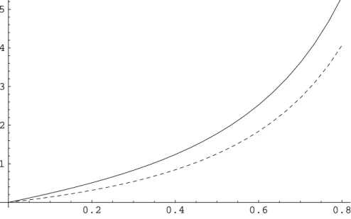
Note that both curves show the existence of an injection point indicated by I on the graphs; however, in casek =;1 (open universe) this injection point is located after the end of conformal time ( > f) and is therefore physically irrelevant. The existence of such a point is only of interest in the case of a spatially closed universe. The obtained curve fork= 0 has the same qualitative features, but for the fact that the injection point moves to the end of conformal time: I =f in that case.
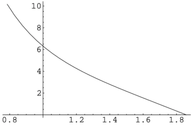
The shape of T(), as given by Figures 4 and 5, is in full agreement with the qualitative discussion given in the previous section. Such plots were already given in [2], where Weierstrass functions had been numerically calculated from the algorithms obtained in the same reference. The same plots can now be easily obtained using, for example, Mathematica, (latest versions of this program include routines for the Weierstrass functions P; and.
Note, however, that intensive computations involving such functions should probably make use of the extremely fast algorithms described in reference [11]; these algorithms use, for the numerical evaluation of these functions, a duplication formula known for the Weierstrass P-function. Therefore, you get a correlation between the values of the reduced temperature T at (conforming) times and 2, which in casek= +1 reads.

Determination of all Cosmological Parameters: a Fictitious Case
- A Simple Procedure
- An Example
The value of the Hubble constant makes it possible to determine all dimensional quantities, in particular the critical length parameter c (formula 17), the cosmological constant (=c), and the current values of the cosmic scale (or \radius" ) Ro (formula 18) and from cosmic time to (formula 19). Here we follow the previous procedure, assuming fully determined values for the Hubble constant and density parameters m and. Such precise values are of course not yet experimentally available and we must make an arbitrary choice (compatible with observational limits) to illustrate the preceding simple procedure leading to the determination of all cosmological parameters of interest.
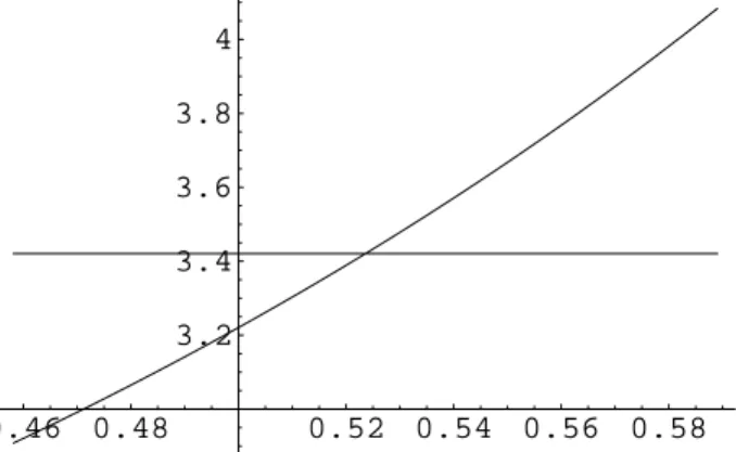
The evolution of the dimensionless temperature is T() = 6P(;fg2;g3g)+1=12 and its current value turns out to be To = 3; this is a strange coincidence (see Section 3.3), since To has no reason, a priori, to be equal to the temperature of the cosmological blackbody radiation ~To. The current value of the conformal time obtained by numerically solving the equation T(o) = This is o = 1:369. The conformal time for which T() has an excision point is obtained by numerically solving the equation T()00= 0 and is I = 1:691.
Note that in that particular universe we have o< I (< f), so we have not yet reached the inexy point. Taking this value into account together with the results from Appendix 1 leads to a slight change in the values ofo and therefore ofto.
5 INFLUENCE OF THE COSMOLOGICAL CONSTANT ON THE REDSHIFT. LARGE SCALE STRUCTURES
Cosmological Constant Dependence of the Redshift Function
Observer Dependence of Redshift Values and Large Scale Geometry of the universe
- Comparison of Measurements Made at the Same Time
- Comparison of Measurements Relative to a Single Event
It is common to specify events with a pair (;S), where S is a point in space (e.g. the Sun) and some value of the conformal time of the universe. Of course, both z and Z are given by the previous general formula, which expresses the redshift as a function of the time difference between emission and reception, but this value is not the same for S and forP. For denitency, we assume that we are in the closed case (k = 1), that is, the spatial universe is a three-sphere S3.
The fact that the universe is expanding is taken into account by developing a reduced temperature as a function of conformal time and, as far as geometry is concerned, we can analyze the situation on a fixed trisphere of radius 1. Choosing a point P { we will call it \Pole", but an arbitrary point { allows defining concepts of the equator and cosmic latitude: relative to P, the equator is a two-sphere (normal sphere) of the largest radius, centered at P and the cosmic latitude'(S) of the Sun S is just the length of the arc of the great circle between S and the equator; this great circle is a geodesic longitude that passes through the two points P and S (which we do not assume, antipodal!). It is also clear that (conformal) time difference = o; between the observation (with S at time o) and the emission of light (with X at time ) there is nothing but the measure of the geodesic arc defined by the two points S and X on the unit trisphere.
The last piece of information we need is a measure of the angle1, as seen from Sun (S) between the direction of P and the direction of X. Returning to our problem of comparing redshifts, we find that is the redshift of the objectX, as observed by P at conformal time o. P of the Universe, around the value Z of the redshift, would certainly be an example of a (remarkable) large-scale structure, but such a gap would become direction-dependent as seen from another point S (the Sun); the previously given formulas will then be needed to perform the necessary modification of redshift maps so that one can recognize the existence of these features.
To simplify the calculation, we assume that S1 and S2 belong to the same meridian (passing through P) of our space hypersphere and call 1 (respectively the redshift z2 of X, measured by S2 is given by the above formula, but since everything else is extrapolated, it becomes just a function of cosmic latitude `(S2). Keeping the same notation as before, the cosmological event of interest occurred at conformal time o;, and the light will reach P at time o;+ =2 ;`(X).
In the case 6= 0 it is of course still possible to express T in terms of y (with the fractional linear transformation 20, with y = P(;g2;g3), the Weierstrass P-function. Such plots have already been given .in [2] where Weierstrass functions were calculated numerically from the algorithms obtained in the same reference In the three-dimensional situation the unit 1 is a specific point of the three-sphere S3 and we will write in the same way.
Finally, the following formula relates the lengths of the three sides of the geodesic triangle SXP, together with the angle: