The importance of key capabilities for generic 5G services
Massive MIMO in Fixed wireless (FW) use case exploiting beamforming
Multipath propagation of a signal
Array steering modeling for Uniform linear array (ULA) assuming planar waves. 12
General transform coding block diagram
Staircase structure of a scalar quantizer
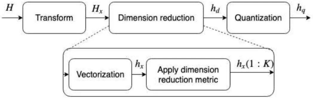
Generic block diagram of the transform coding methods evaluated and proposed
Algorithm for implementing Discrete cosine transform (DCT) or Discrete Fourier
Algorithm for implementing DCT or DFT Signal to noise ratio (SNR) target
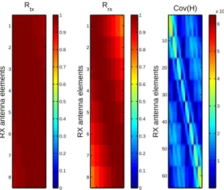
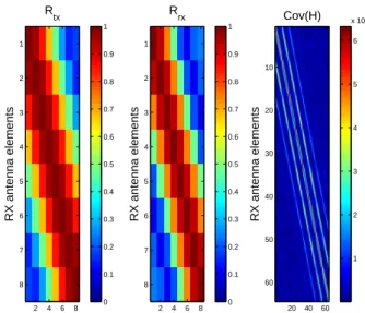
Parameters used to model the covariance matrices at transmitter and receiver of
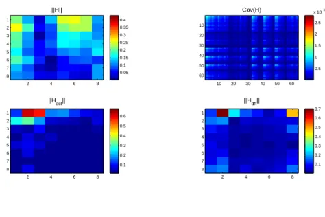
Covariance matrices for the Kronecker channel model with antenna element
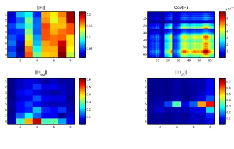
Covariance matrices for the Kronecker channel model with antenna element
Dissertation outline
Thus, the overhead of open-loop channel acquisition is the product of the number of training pilots on the uplink, which is proportional to the number. In closed-loop MIMO, the downlink training overhead is independent of the number of users, but proportional to the number of transmitter antennas Ntx [10].
MIMO propagation characteristics
9 antennas in each UE, and the number of users participating in the uplink channel ringing CSITDD ~ NUENrx [18]. The overall cost for the uplink is proportional to the number of scheduled users multiplied by the size of the channel matrix, which is the product of the number of transmit antennas in BS Ntx and the number of receive antennas in each UE Nrx [ 18 ]. Therefore, FDD feedback is proportional to CSIFDD ∼ Ntx +NUENrxNtx, which requires precious transmission resources, leading to the interest to compress feedback data.
Thanks to advances in the electronics industry, MIMO can reach a huge number of antennas within frequency bands in the 30-300 GHz range, known as mmWaves. Measurement campaigns of sub-6 GHz massive MIMO have shown that increasing the number of antenna elements leads to UE channels being nearly orthogonal.

MIMO channel modeling
Narrowband multipath channel model
If we know the array steering vector, the multipath narrowband model for the array channel matrix is.
Narrowband Kronecker channel model
When the energy dissipated in the receiver is assumed to reach a uniformly distributed range of angles, the covariance matrix of a ULA can be calculated as . Assuming that the distance from the transmitter to the receiver is greater than the antenna spacing, the angle of arrival and the angular extent for a ULA can be calculated as [25, 26]. In general, an increase in antenna element spacing causes Rrx and Rtx to become more diagonal, therefore the antenna elements are less interconnected [16, 25].
14 spacing increases, decreases the electromagnetic coupling between the antenna elements leading to less correlation between antenna elements [16]. In this scenario, the signal at each receiving antenna is the same and the antenna elements are perfectly correlated as long as electromagnetic coupling is negligible.

MIMO channel sparsity
These operations are reversed at the decoder, where an approximation of the input sequence is reconstructed [28]. The original purpose of transform coding is to extract the redundancy that exists between elements of arbitrary vectors, such as in a multi-channel environment with cross-coupling between channels or in arbitrary vectors formed by blocks of consecutive samples of a scalar signal, by applying a transform and then quantize the value. transformed vector [29]. At the encoder, the direct linear transformation of the sampled input signal
Hence, AH is the direct transform matrixΨxenAis the inverse transform matrixΨxH so that the columns of Ato contain the basis vectors of the transform [29]. The transformation coding gainGT C measures the energy density of a given transformation and is calculated as.
Signal processing for sparse signals
- Karhunen-Lo´eve transform
- Discrete cosine transform
- Discrete Fourier transform
- Compressive sensing
According to [31, 32], DCT asymptotically approaches KLT performance for highly correlated (Markov-1) processes, regardless of the size N of the signal sequence. This repetition of the sequence at each point M causes sharp discontinuities at the edges of the sequence leading to high frequency components. However, the sparsity of K can be exploited where y is simplified to a combination of K columns of Θ.
As K ≤ M, the system M × K is well-conditioned if Θ preserves the length of K sparse eigenvectors [35]. From this, the elements of the measurement matrix Φ can be generated from random variables with Gaussian or Bernoulli distribution, and Θ=ΦΨxhas to present the restricted isometry property (RIP) [35, 36].
Side information
Therefore, a significance map always needs the same number of bits, which coincides with the total number of coefficients. When an RLE encoder detects a long string of the same value, it indicates that specific value and the number of times it occurs. Encoding a series of bits 0 or 1 requires bits that represent a certain range of integers.
For example, a run of 150 bits of zero would require 8 bits to represent the number of occurrences. Unless entropy coding such as Huffmans code is used, the number of bits required to represent the maximum drive will be needed each time a bit is flipped from 0 to 1 or vice versa.
Quantization
Scalar quantization
Associated with each M-point quantizer is a partition of the real line R into M cells or atoms Rifori = 1,2,. The total length of the grain cells is called rangeB, where for an unbounded proper quantizer, B =xM−1−x1. Nevertheless, the load factor measures the magnitude of the maximum decision level xM−1 with respect to the root mean square (RMS) value σ of the input signal.
For the case of a symmetric quantizer, V =B/2, where B =xM−1−x1 is the total length of the grain cells. A uniform quantizer is the simplest type of quantizer, where all intervals are the same size, except for perhaps two outer intervals that may form an overdrive region.

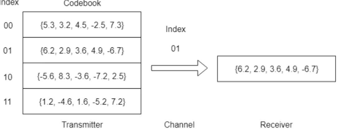
Vector quantization
Compared to scalar quantization, VQ gives flexibility to represent the source outputs; furthermore, if the source results are related, this structure can be explored to create effective representations. LBG is very similar to the k-means algorithm from pattern recognition applications, but differs in terms of initialization [30]. When all elements are assigned, the codewords are updated by computing the centroids of the training set vectors assigned to them.
When the assignment process is complete, there will be M new groups of vectors clustered around each of the output points, the code vectors [30]. Both LBG and k-means algorithms guarantee that the distortion will not increase from one iteration to the next.
Compression metrics
28 where σx2 is the root mean square value of the source signal (zero mean signals are assumed below, unless otherwise stated). This dissertation adopts two metrics, the first is called the compression ratioη, which concerns only the number of discarded coefficientsNdiscarded, disregarding quantization, and is given by. CF and η can be used for a single realization of the channel array or in an average sense.
One can also separate the numerator and denominator of CF and interpret CF as the ratio of the average number of bits to the coefficient of the channel matrix.
CSI compression for limited rate feedback
The method relies on a power factor which defines a zero-one filtering matrix, which will further be used to discard coefficients of the DCT-transformed channel vector; the filtering matrix is sent as page information to the transmitter. However, the method proposed in [44] is computationally difficult because it operates VQ coding on the UE side, which has relatively high computational cost. This adaptive method uses DCT as the sparsification basis, and the method overhead is to inform the transmitter of the values of M.
Despite the reduction in feedback, the method assumes that the UE simulates the recovery process to handle the KLT base update, which increases the complexity at the receiver side. Moreover, the method is limited to slow changing conditions which may not happen in many 5G scenarios.
Proposed low-complexity CSI transform coding
- Sparsifying transform
- Determining the relevant coefficients based on target distortion
- Encoding few relevant coefficients
- Quantization
- Simulation of Kronecker channel model
- Ray tracing (RT) simulation and multipath channel model
From the previous example, the indices hs I and side information to restore the position of the quantized coefficient Is={4,2}. 36 matrix and imaginary part quantizer are designed with the same amount of bits. One thousand realizations of the channel matrix are generated from equation (2.6) and the mean covariance matrix of the final channel is calculated.
This reduction of correlated pixels on the final covariance matrix will further affect the performance of the compression methods presented in Chapter 3. It can be noted that the boxplot is mostly concentrated around the average delay value for most of the receivers on the analyzed episodes.
Analysis of channel model and orthogonal transform
Transform analysis of Kronecker channel model
Note that the covariance matrices R from the Kronecker channel model are not calculated here because RT is a deterministic simulation approach.
Transform analysis of RT dataset at sub-6 GHz
Figures 4.18 and 4.19 show the energy compression to apply DCT and DFT to the 60 GHz FW Raymobtime dataset with multipath channel model post-processing with 0.1λ and 0.5λ antenna spacing, respectively. Figures 4.22 and 4.23 show the energy compression to apply DCT and DFT to the 60 GHz V2E Raymobtime dataset with multipath channel model post-processing with 0.1λ and 0.5λ antenna spacing, respectively. This decrease in the compression factor as the antenna distance increases is noted in all compression metrics in Figure 4.25.
From Figure 4.27, it can be observed that the target DFT SNR method has higher compression factor for λ = 0.5 than for dλ = 0.1, this shift does not occur in the Kronecker channel model data set. The SNR results for the FW use case operating at 60 GHz are shown in Figure 4.28 and CF.
Transform analysis of RT dataset at Millimeter waves (mmWaves)
Evaluation of compression metrics
Compression ratio
For the Kronecker channel model, the compression ratio varies significantly when the antenna spacing increases from 0.1λ to 0.5λ; such an effect can be explained by the reduction on channel correlation shown in Figures 4.2 and 4.3. Moreover, DCT becomes the best choice for both antenna spacing, in this case, due to the covariance structure of the Kronecker channel model. For the Raymobtime dataset, DCT also allows better compression when the antenna spacing is 0.1λ; however, when the channel spacing increases to 0.5λ, DFT has a better compression ratio for either FW or V2E use cases.
Furthermore, the compression ratio achieved by DFT is quite stable to changes in antenna spacing, while DCT suffers about 6% reduction in its compression performance when the antenna spacing increases from 0.1λ to 0.5λ. The stability in DFT compression performance may also be an effect of the direction vectors used to model the linear arrays in the multipath channel model, because the direction structure is similar to a DFT matrix.
Signal to noise ratio and compression factor performance
Considering the design benchmark of achieving 6 dB SNR with the least number of bits, the SNR target method using DCT would be chosen because its performance requires the least number of bits and does not go below the SNR target as the antenna distance gets bigger. Therefore, the chosen transform coding for this case is the SNR target using DFT, as it uses the least amount of bits and provides good performance in both antenna spacing scenarios. By analyzing both graphics together, the SNR target with DFT also provides a good trade-off between the number of bits required and the achieved SNR for both antenna spacing scenarios.
In this scenario, the SNR target with DFT is also the chosen method for transform coding, given the higher SNR performance and reasonable number of bits required in both antenna spacing scenarios. For example, this work highlighted that the antenna spacing has a significant impact on the compression results.

Published Articles
Sayeed, “A review of signal processing techniques for millimeter wave MIMO systems,” IEEE Journal of Selected Topics in Signal Processing, vol. Kahn, “Fade correlation and its effect on the capacity of multi-element antenna systems,” IEEE Transactions on communications, vol. Pearl, “Comparison of cosine and fourier transforms of markov-1 signals,” IEEE Transactions on Acoustics, Speech, and Signal Processing, vol.
Transform Coefficient Coding in HEVC," IEEE Transactions on Circuits and Systems for Video Technology, vol. Andrews, “A Review of Limited Feedback in Wireless Communication Systems," IEEE Journal on Selected Areas in Communications, vol.