In particular, if f and g are potentially positive L-functions, exactly one of the following relations holds. A function p is a zero-one law if and only if all models of the almost certain theory Θp are elementary equivalent.
The Ehrenfeucht-Fra¨ıss´ e Game
We then transform K into a topological space by treating sets of the form Aφ={[H]∈ K |H |=φ} as basic open sets. Each node T is a pair (A, h), where A is a nonempty closed set and h∈Ni is the height of the node.
Borelian Probabilities on K(Θ)
Application to Random Hypergraphs
Counting of Berge-Tree Components
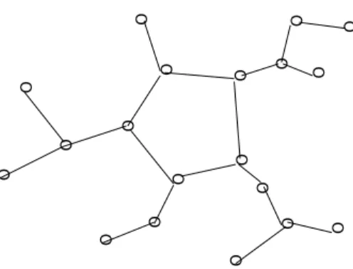
Given the above, as far as all our current discussions are concerned, the hypergraphs we deal with are disjoint Berge-three unions. Below τ ∈ T, where is the set of all isomorphism classes of Berge trees of order lon v= 1 +ld labeled vertices. Let cτ(l) be the number of Berge trees of class orderl and isomorphism τ in v= 1 +ld labeled vertices.
XScτ(l), each indicating that one of the potential cτ(l) Berge trees of order l and isomorphism class τ in S is present and is a component. Next, we show that a local threshold for containing a Berge tree of given order as a connected component is the same for containing Berge trees of that order as sub-hypergraphs, not necessarily induced. The function vl is a local threshold for inclusion of Berge trees of order l as components.
Let Θl be the first-order theory consisting of a scheme of axioms ruling out the existence of cycles and Berge trees of order ≥l+ 1 and a scheme ensuring the existence of infinite copies of each type of Berge trees of order ≤l.
Just Before the Double Jump
We refer the reader to [13] for the proof of the above claim, which is a direct application of the first and second moment methods. Note that by the above proposition, all the countable models of the almost certain theory Θp are isomorphic, i.e. Θp are ℵ0-categorical. Let H1 and H2 be two acyclic graphs where each finite Berge tree appears as a component an infinite number of times.
It is convenient to emphasize that H1 and H2 may or may not have infinite components. Let Θ be the first-order theory consisting of a scheme of axioms that excludes the existence of cycles and a scheme that ensures that every finite Berge tree of any order appears as a component an infinite number of times.
On the Thresholds
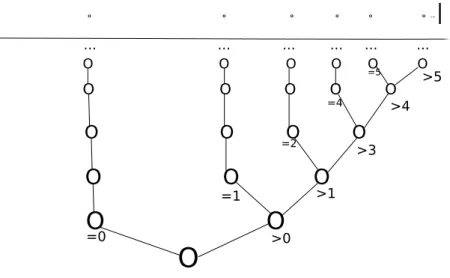
It is worth noting that ifai is the number of automorphisms of the Berge tree whose isomorphism is of type isτi, then one has cv!i = a1. The convergence laws we have obtained so far provide a nice description of the constituent structure in the early history of Gd+1(n, p): it starts empty, then isolated edges appear, then all Berge trees of order two, then all of order three, and so on to n-d, just before the double jump occurs. It is worth noting that the arguments used in deriving zero-one laws for intervals.
We also note that, in a sense, most functions in WB are zero-one laws: the only way one of those functions can avoid this condition is to be inside one of the countable windows within a threshold representation of Berge trees . of some order. In the following sections, similar pieces of reasoning will yield an analogous result for another range of edge functions. We call that interval BC, for Big-Crunch, because, informally, when "time" (the p-edge functions) flows forward, the behavior of the giant component's complement is the same as that.
Within the window p ∼ C·(logn)n−d (with C a positive constant), much the opposite is true: here we find an infinite set of local thresholds of elementary properties and also an infinite set of zero- one and convergence laws.
Just Past the Double Jump
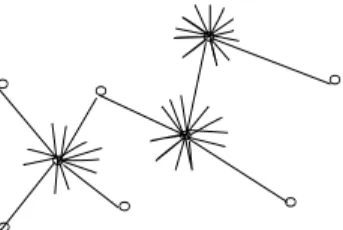
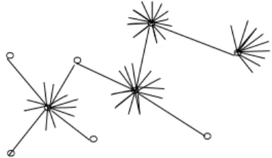
Now it is easy to see that the edge functions in the current series are zero-one laws, which gives part (1)(d) of 1.1. According to Theorem 5.1, every vertex in the union of all the unicyclic components has infinite neighbors. But in the complement of the above set, we have already seen that Duplicator can win all k-round Ehrenfeucht games.
We note that the non-existence of small-degree vertices near cycles is first-order axiomatable. For every l, s, k ∈N there is a first-order sentence that excludes all (finitely many) configurations with cycles of order ≤ l at distance ≤ s from one vertex of a degree. Similar considerations show that the non-existence of bicyclic (or more) components is also first-order axiomatizable.
Thus, one easily gets a simple axiomatization for the almost certain theories of the above fringe functions.
Beyond Connectivity
It determines these components to isomorphism and it does not pay for Spoiler to play there. Again, the thresholds for the appearance of small sub-hypergraphs imply that, in this series, we have all cycles of all types as sub-hypergraphs, and no bicyclic (or more) components. The countable models of Θp have components containing cycles of all types, no bicyclic (or more) components and may have Berge-tree components.
Since no vertex can have a small measure, all vertices in that component have infinite neighbors, so these components are unique up to isomorphism. The results regarding winning strategies for Duplicator mentioned before give that these models are elementally equivalent, so they are zero-one laws. The discussion found on the proof of Theorem 5.4 also gives simple axiomatizations for the almost certain theories of the above p.
Marked Berge-Trees
Now, the most important concept to understand the zero-one and convergence laws on BC is the counting of minimally labeled Berge trees. Let Γ be the finite set of all isomorphism types of minimal v∗-labeled l-Berge trees on 1 + ld labeled vertices and set γ ∈ Γ. Then c(l, v∗, γ) is the number of possible v∗-labeled l-Berge trees of isomorphism type γ on1 +ld-labeled vertices.
More informally, when the coefficient of logndn inp avoids the rational value vd!∗ then the expected number of Berge trees denoted by v∗ is either 0 or. The second-moment method will give that, in the second case, there are many such minimal marked Berge trees. If this coefficient avoids the integer value l, then the expected number of l-Berge trees denoted by v∗ is either 0 or.
Again, first and second moment arguments imply that, in the first case, the number of such Berge trees a.a.s.
Zero-One Laws Between the Thresholds
More precisely, the countable models of Θp satisfy the hypothesis of Theorem 2.8, so they are pairwise elementary equivalent and so Θv∗ is complete and the corresponding p are zero-one laws. Ifω → −∞then the first and second moment analysis above imply that the countable models of Θp are the same as the countable models of Θv∗ and, since Θv∗ is complete, pisses a zero-one law. If ω →+∞ then the first and second moment analysis above imply that the countable models of Θp are the same as the countable models of Θv∗−1.
Θlv∗ := Θp are the same as the countable models of Θv∗ but without the components with marked Berge trees of order ≤ l −1. For the same reasons, these models are still pairwise elementary equivalent, so we have that the corresponding p are zero-one laws. Ifc→ −∞, then the analysis above shows that the countable models of Θp are the same as the countable models of Θlv∗, so these share zero-one laws.
Čec→+∞, then the above analysis shows that the countable models Θp are the same as the countable models Θl−1v∗, so they also separate the zero-one laws.
Axiomatizations
On the thresholds
The situation is analogous to that of the last section: at these thresholds, the spaces K(Θp) admit weighted spanning trees. Indeed, the union complement of the components containing the Berge trees denoted by v∗ of order is elementary equivalent to the countable models of the theory Θl+1v∗, defined above. Arguing as in proposition 5.13, it can be seen that the contribution of each of the terms in P.
As was the case with BB, our current discussion implies that, in a sense, most of the functions in BC are zero-one laws: the only way any of those functions can avoid this condition is to be inside one of the countable windows . within a local threshold for the presence of marked Berge trees of a particular order. Simple applications of Theorem 2.2 imply that, in this range, the countable models of the near-certain theory have infinitely connected components isomorphic to any finite Berge tree and have no bicyclic (or more) components. The above considerations suggest that it may be useful to consider the asymptotic distribution of the different types of monocyclic components in Gd+1(n, p).
Now, the structure of the set of possible completions of an almost certain theory is more complicated: it is a Cantor space.
Values and Patterns
Also, any rooted Berge-tree can be treated as a uniform hypergraph if we remove the special label of the root. Then pnΓ is the probability that the sphere with center v and radius r is a Berge tree with value Γ, taking v as the root.
Poisson Berge-Trees
Size of Neighborhoods
For the induction step, first note that the induction hypothesis implies that almost certainly every ball of radius r has at most one size. We use the method of factorial moments to show that the distributions of the different (r, s) patterns are asymptotically independent Poisson with means λl!l ·p∆i, for 1≤i≤N, which is obvious. First we show that the expected number of pairs of sides Ei, Ej on v1 with patterns ∆i and ∆j are asymptotic to (l!)λ2l2 ·p∆i·p∆j, respectively.
Define ˜pn0 as the probability of event B that the pattern of Ei is ∆i and the pattern of Ej, not counting the vertices already used in Ei. Similar arguments show that, by defining the (r, s) pattern of a cyclic configuration C in the obvious way, the distribution of cycles of the different types is asymptotically independent Poisson. Since none of the branches in this tree are isolated, K(Θp) has no isolated points and is therefore a Cantor space.
The convergence laws in the Double Jump are the last piece of information to 1.1.