In this thesis, the design of quasi-satellite orbits in an elliptically constrained three-body problem is considered from a preliminary perspective of space mission design. The stability of these orbits is studied using an analytical and numerical approach, and the findings are applied to the study of the Mars-Phobos system.
List of Acronyms
List of Symbols
1 Introduction
Motivation
However, the first mission to focus exclusively on Phobos did not take place until 1988 – the Russian probes Phobos 1 & 2. A successful mission to Phobos has yet to be accomplished, with such a mission again described as a major milestone to be overcome (Marov et al., 2004).
Problem Statement
The main and corresponding orbital parameters of Mars and Phobos are shown in Table 1.1. The search for sufficiently stable QSOs with analytical and numerical approaches is the main topic of this work.
Quasi-Satellite Orbits
The exploration of this time dependence in moons orbiting with a small eccentricity, such as Phobos, is one of the main goals of this work. However, the oblateness of Mars and Phobos' irregular shape and rotation is not taken into account - this work was developed under the point mass approach for both bodies.
Stability
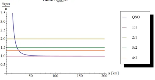
Resonant orbits are any orbits that form with the second primary (in our case Phobos) a system revolving around the same primary (Mars), whose mean orbital motions are proportional to small integers (Peale, 1976). As the orbital amplitude of a QSO increases, the orbit tends to a 1:1 resonance, often called a quasi-synchronous orbit, while at close range fairly stable 2:1, 3:2, and 4:3 resonances can be found (Wiesel , 1993).
Bibliographic Review
- Orbits In The Three-Body Problem
- Chaos Indicators
The study of orbital stability in the three-body problem is one of the most studied topics in celestial mechanics. Most of the CIs based on the analysis of the deviation vector are derived from the LCEs.
Thesis Overview
The variational equations of the Hamiltonian formulation are presented, and the CIs of interest—the LCEs and FLIs—are introduced at the end of the chapter. Furthermore, the theory behind CIs and the method for calculating the CIs of interest are discussed.
Classical Mechanics
- Lagrangian Mechanics
- Hamiltonian Mechanics
- The Variational Equations
The dimension of the configuration space is also called the number of degrees of freedom of the system. The parameters used to specify the configuration of the system are called the generalized coordinates.
The N-Body Problem
The analysis of the deviation vector forms the basis for most CIs, using the concept – introduced by Lyapunov – of exponential divergence, that is, initially nearby chaotic orbits decay roughly exponentially with time, while nearby regular orbits roughly linearly separate with time. time. The kinetic energy of the system is given by the sum of the products of the mass and the squared velocity of each particle. 2.17) The Hamiltonian of the system is the sum of the kinetic and potential energies.
The Restricted Three-Body Problem
The first body with mass 1−µ is fixed in the reference frame at (µ,0), and the second body with mass µ is fixed in the reference frame at (µ−1,0). Changing the velocities in the Lagrangian gives the Lagrangian in the synodic or rotating frame LR= 1.
Modifications of the Restricted Three-Body Problem
- The Spatial Restricted Three-Body Problem
- The Elliptic Restricted Three-Body Problem
- Change Of Origin
This equation derives from the principle of conservation of angular momentum of two primaries. The expansion in the three-dimensional case is straightforward, but note that while the third coordinate does not occur in the transformation involving rotation about the z axis, it is made dimensionless by the variable distance between the primaries and also takes on a pulsating character. Studying the problem in this new frame of reference has several advantages for the analytical treatment of the problem, since the coordinates (ξ, η, ζ) are small when compared to the unit length.
We work in a synodic frame of reference centered at Phobos, with the x-axis pointing to Mars, the z-axis pointing to the direction of Phobos' angular momentum, and the lateral axis completing the right-handed orthogonal system.
Equations of Motion
- Hamilton’s Equations of Motion
- An Invariant Relation
In the circular problem, which is described by autonomous equations, the integral on the right-hand side of equation (2.56) is immediately deduced to be 2Ω−C. Therefore, the right-hand side of equation 2.56 can be written as 2.60) To consider a path for a short time, which means that we choose the time to start the movement at, e.g. f = 0, and we are only interested in the part of the trajectory that takes place between f = 0 and f = where is a sufficiently small positive quantity. Since f is the true anomaly, this restriction corresponds to considering a sufficiently small time interval in which the primaries describe sufficiently small arcs.
The second term on the right-hand side of (2.60) in this case contains the product of the eccentricity and is consequently smaller than the term2Ωe.
Chaos Indicators
- Lyapunov Characteristic Exponents
- Fast Lyapunov Indicator
We also review the calculation method for mLCE, which is useful for defining the FLI calculation method. The knowledge of the spectrum of the LCEs provides the basic information about the behavior of a dynamical system. We now define the local expansion coefficient of the deviation vector, αi, for a time interval τ when.
In some definitions, FLI can also distinguish resonant from non-resonant motion (Skokos, 2010).
3 QSO Solutions and Stability
Linearization of the Equations of Motion
It is much better to predict without certainty than not to predict at all. If we assume that the second primary mass is much smaller than the first one, i.e., μ <<1, equations (3.3) can be simplified even more. The assumption that the third body is in the vicinity of the second primary gives r2 << 1(with x, y, z << 1) and, thus, the terms that are multiplied by μ and not divided by mer32 can be neglected because they are too smaller than the remaining terms.
Equations (3.4) are the usual form of equations of motion for the spatially elliptic restricted three-body problem to study orbits near the second primary with dimensionless mass µ <<1.
Unperturbed Hill’s Equations
- Homogeneous Solution
- General Solution
- Stability Considerations
- Constants of Integration
- Constant Transformation
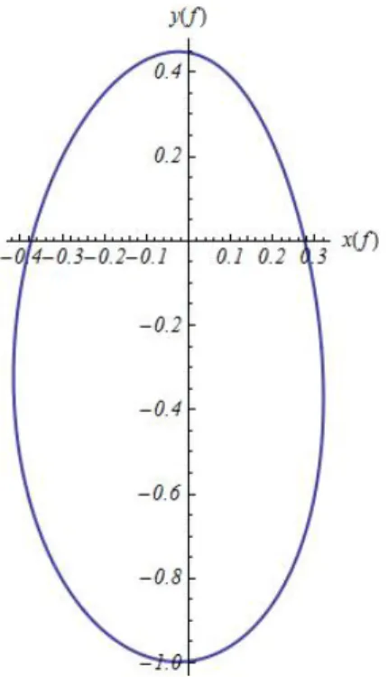
The practical significance of the above definition is that the stability condition (3.25) allows for small shifts in the initial conditions affecting C2 and C3. For a z-coordinate whose solution is independent of the other two coordinates, calculating the constants is a trivial task. The center of the orbit is shifted along the xandy direction by δx (zero for the undisturbed case) or δy, respectively.
Finally, the contour of the path lies in a plane which intersects the xy plane along a line.

Influence of the Second Primary
- Region of Stability
- Approximate Solutions in the Osculating Elements
Elliptic integrals of the first and second kind, respectively F(θ, k) and E(θ, k), with amplitude of the modulus and will be defined as (Gradshteyn and Ryzhik, 1994). The following properties (Gradshteyn and Ryzhik, 1994) are important in our derivation of the mean terms. The method of variation of arbitrary constants is used to obtain the approximate solutions in the osculating elements.
Consequently, the inclination of the QSO also affects the recovery capability of the second primary.
Application to the Mars-Phobos System
Analytically, the period is infinite for the discarded orbits, therefore, the quantity qcc can be calculated numerically by finding the root of the denominator in (3.82). The periods of the osculating elements are, in function of the dimensional amplitude (in kilometers). The relationship between the mean orbital motions of the QSO and Phobos can also be studied through equation (3.80).
From (Wiesel, 1993) it is known that sufficiently stable resonance paths exist for these values of the ratio nQSO/n.

4 Numerical Exploration of QSOs
Numerical Integration
Implementation Validation
- Validation Test
- Implementation Language
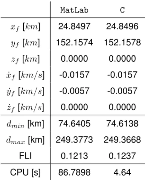
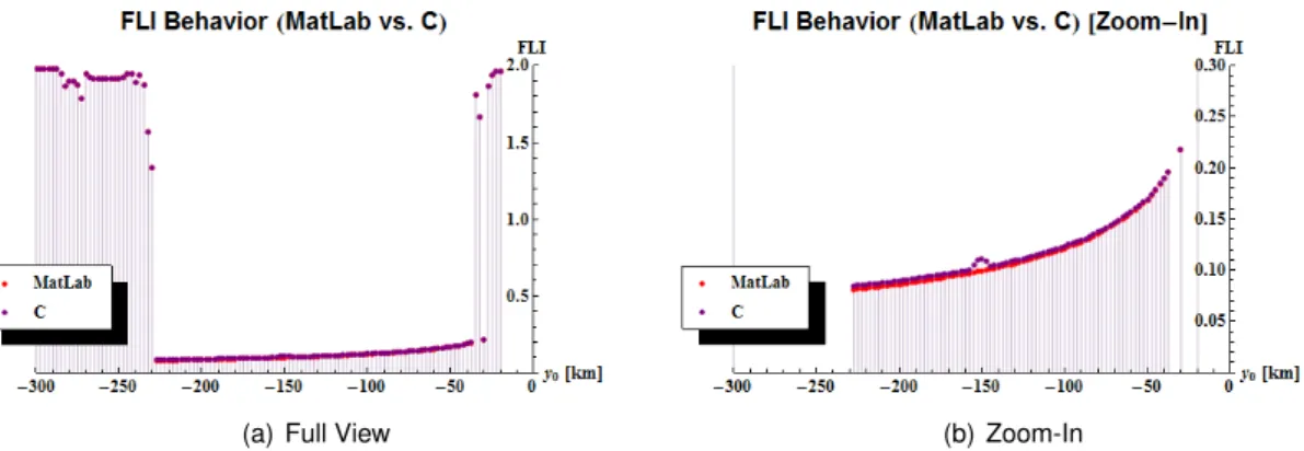
The implementation inCis proved to be much faster in the calculation of FLI. The comparison of the two implementations is performed with a sample path in our problem. The final result of FLI is not important, only its behavior for different trajectories ie. its ability to distinguish chaoticity.
Although there is a small difference in the absolute value of FLI, the results presented in Figure 4.1 show that FLI maintains its behavior in both designs.
Computational Parameters & Methodology
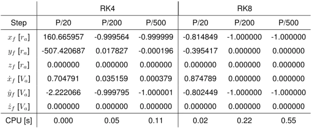
- Integration Method and Time-Step
- Orbit Escape
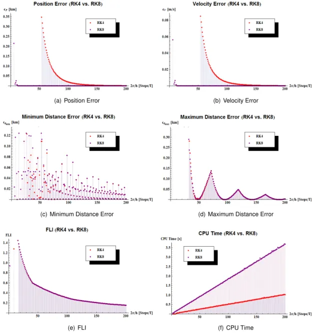
Note that the performance values are evaluated as functions of the number of integration steps per period2π and not directly as functions of the time step. Figures 4.2(a) and 4.2(b) present a plot of the error in these parameters versus the number of steps per period for both methods. The results suggest that 16 steps per period are sufficient for RK8 to meet the defined thresholds.
The two objectives of the numerical exploration are to obtain the solution of trajectories and to assess which of these are sufficiently stable by studying the deviation vector.
FLI Maps
- Planar QSOs
- Three-Dimensional QSOs
- Velocity Maps
The characterization of the FLI maps as a function of the modified Jacobi integral provides insight into the sensitivity of the stability regions to the initial conditions. The initial velocity x˙0 is derived from the defined value of the initial value of the modified Jacobi integral. We are interested in the analysis of changing initial height with changing speed.
Three-dimensional QSOs present a different behavior for large values of the amplitude in the x-y plane, α.

5 Conclusions
A study of resonant orbits is also needed, as these represent the stable, lowest-altitude orbits for Phobos and are mainly of interest for approach or close observation orbits. In the Mars-Phobos system, it is possible that chaotic regions can be found at distances close to the libration points, just above the lunar surface. A future study on transfer paths between QSOs and the respective optimization would also be an asset.
These moons are known to be potential targets of future missions and the study of their orbital mechanics is of benefit to mission designers.
Bibliography
L.: 1989, Distant satellite orbits in the restricted circular three-body problem, Cosmic Research (Translation by Kosmicheskie Issledovaniya. A.: 1993, Theory of perturbations and analysis of the evolution of quasi-satellite orbits in the restricted three-body problem, Kosmicheskie Issledovaniia31, 75-99 Lyapunov, A.: 1992, The general problem of motion stability, Control Theory and Applications Series, International Journal of Control edn, Tayor & Francis.
M.: 2011, Comparison of different chaos indicators based on deviation vectors: application to symplectic mappings, celestial mechanics and dynamical astronomy.