Thermodynamics and information in linear quantum lattices

In this case, the phonons are responsible for the propagation of heat, and by measuring its average occupation number in the steady state, one can determine the type of transport of the system [18]. Thus, the question is more appropriately phrased in terms of the amount of information shared between different parts of a quantum chain.

Postulates of Quantum Mechanics

It can be shown that such complicated interactions can be described by a set of measurements performed on the system. The area of ​​quantum mechanics that studies the evolution of subsystems in contact with an environment (that is, a set of other quantum subsystems) is commonly called open quantum systems [51].

Quantum master equation

For the interaction term, we will assume that the system-environment coupling is linear4in bα,k. We will consider that the initial state of the system is uncorrelated with the bath, i.e.

A simple example: One mode coupled with a bath

The Covariance Matrix

2.16), we can calculate the time evolution of the average value of the number operatorO=a†a. which has an exponential decay as a solution, To illustrate the CM form, we write the case of two modes (L=2) and the first vanishing moments (µ=0):.

Time evolution of the Covariance Matrix for short range Hamiltonians

For completeness, we mention that the 2L block matrix G in Eq. (2.41) can be written in terms of the reduced matrices FN and FM as Now, to provide a better understanding of the physics behind this model, we briefly review here some basic notions of typical transport problems arising from non-equilibrium processes.

Solution of the Lyapunov equation in the Non-Equilibrium Steady State

3.6) is now formally identical to the model studied in Refs. 40-42], which instead of using self-consistent baths, used mold dephasing baths. The NESS of the self-consistent reservoirs is Gaussian, but that of the dephasing model is not. We also mention that the self-consistent model can be easily expanded for the case of squeezing, while the dephasing model cannot, since a dissipator as in Eq. 3.7) maintains the number of particles, but does not maintain the level of squeeze.

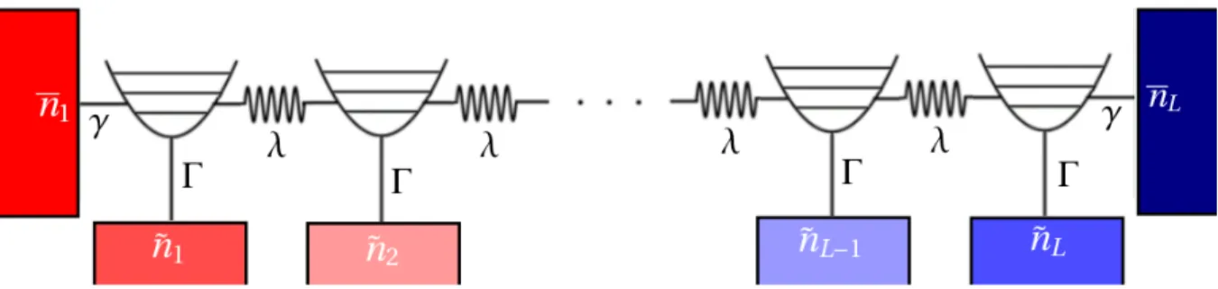
To achieve diffusion, the system has been expanded with self-consistent reservoirs, one for each place in the chain.

The current

E = 0 and because the particles are a conservative quantity, the current entering the system is the same as leaving,JB,1 = −JL,B4. No, the current from thek-th mode to thek+1-th is equal to the current from thek−1-th to thek-th,. Once this work term is identified, it appears (for the specific case of a bosonic chain) that the current of Eq. 3.18) will also correspond to the heat flow to the baths, up to a constantω.

It is worth noting that the current depends on the gradient of the occupation number, as it depends on the temperature gradient in Eq.3.1.

Ballistic vs. di ff usive transport

General NESS covariance matrix with squeezing

The entropy production rate is always non-negative and is zero if and only if the system is in equilibrium, which is a consequence of the second law of thermodynamics. When the system is allowed to relax in contact with a single reservoir, it will generally reach thermal equilibrium where dS/dt = Π = Φ = 0. However, when the system is connected to several reservoirs held at different temperatures , it will instead reach a non-equilibrium steady state (NESS) where dS/dt = 0 but Π = Φ ≥ 0.

Within our phase-space formulation, we are able to obtain expressions that clearly illustrate this interplay between irreversible quasi-probability currents, resulting from the contact with the reservoirs, and unit currents, resulting from the internal system interactions.

Phase space: the Wigner function

We are then able to quantify the individual contributions to irreversibility originating from the physical reservoirs and that originating solely from the self-consistent baths.

Quantum Fokker Planck equation

Wigner entropy production of each dissipation channel

First and foremost, it is clear that the rate of entropy production is always non-negative and equal to zero if and only if the fluxes themselves are always equal to zero, which only happens in equilibrium. Second, the entropy production rate is said to be an even function of irreversible fluxes, while the entropy flux rate is found to be an odd function, as found in other studies of the Fokker-Planck equations [88]. In particular, the entropy production rate (4.20) gets an interesting and rich physical interpretation due to its connection with microscopic irreversible flows Jk(W).

The entropy production rate (4.20) can also be expressed in terms of the covariance matrix of the system, similar to the flux (4.23), although the expression is not as simple.

Role of the unitary dynamics in maintaining a non-equilibrium steady-state

If the mode has a higher occupancy than the environment, we get Φk > 0, which means that entropy flows from the system to the environment. Conversely, if ha†kaki < n¯k, then Φk <0 and entropy will flow from the environment to the system. The first term, Πtrans, due to a transient, can be found in many studies of entropy production and usually involves an interpretation in terms of the rate at which the system approaches equilibrium (with the relative entropy playing the role of the distance between the current state and equilibrium state).

When they do, the system will instead reach a NESS, where the first term is zero, but the second term remains despite. 4.29) proves the essential role of the untary interactions in allowing currents to flow from one bath to another, maintaining NESS and a limited entropy production rate.

Recovering Onsager’s theory of irreversible thermodynamics

Within this framework, entropy production is defined as the product of fluxes times affinities (also called generalized forces). The non-negativity of the entropy production rate is reinforced by the fact that the current always flows from hot to cold, so that the sign of jAB will always be the same as TA−1−TB−1. 3It is more general because we use the Hamiltonian of Eq. 2.4), which does not allow for local correlations. Thus, the production rate of entropy is clearly always non-negative and zero if and only if.

It is also noteworthy that when fixing the temperature gradient, the ballistic irreversible entropy production rate ΠNESS(γ,Γ =0) is greater than the diffusive enΠNESS(γ,Γ> 0).

Entropy production rate from the physical and the self-consistent reservoirs

Here we have already made use of the fact that the occupation number of the self-consistent reservoirs is formed to be ˜nk =ha†kaki, so that the entropy flux of the self-consistent reservoirs ˜Φk, disappears. Instead, the question is more appropriately phrased in terms of the amount of information shared between different parts of a quantum chain. This competition between heat currents and decoherence will eventually produce a NESS where different parts of the chain share a certain amount of information with each other (see for example Ref. [105]).

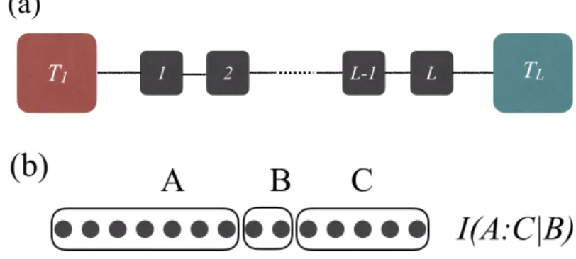
For a connected bipartition of the chain, the natural quantifier is the mutual information (MI).

Quantifying the information sharing

In this chapter, however, we will mainly focus on quantifying the information that is shared between two disconnected parts of the chain. But instead of a probability distribution P(X,Y,Z) we now have a multi-site density matrixρof the NESS. Despite this difference, the logic remains the same: the ability of the flows to share information between A and C is correctly captured by the CMII (A:C|B) and not by the MI.

If I(A :C|B) = 0, then no information is shared, while the dependence of I(A:C|B) on the size of eB determines the robustness of the chain in information sharing, regardless of the noise in the channel.

Calculation of the entropy

Analysis of the shared information in a Non-Equilibrium Steady State

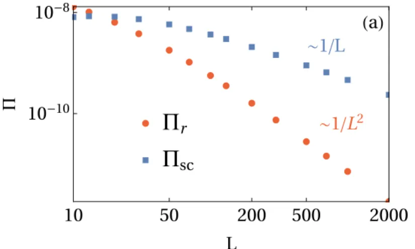
I−1/(2b+2)vs.ΓLfor different values ​​ofΓ,Landb. 6.11), this should lead to a fully collapsed straight line, which is exactly what is observed. 6.11) provides a complete characterization of the information transport for the bosonic model described in Chapter 3. It shows that the information transport is suppressed exponentially by the size b of the middle partition, for both ballistic and diffusive cases. In the diffusive case, however, this suppression is greatly enhanced by a factor that depends on the size L of the chain.

116], where in certain cases the NESS can be in a product state, despite a non-zero current.

Local equilibration

We have addressed the computation of the irreversible rate of entropy production using a quantum phase space approach based on the Wigner entropy. First, we have shown that conditional mutual information emerges as a strong quantifier of the ability of Let us begin this demonstration by writing the R´enyi-2 entropy in terms of the system purity P,.

First, we get an expression that relates the purity to an integral of the Wigner function.

The purity and the Wigner function

For Gaussian systems, R'enyi-2 entropy satisfies the strong subadditivity inequality [115], and can be used as a suitable tool to calculate information-theoretic quantities. Second, we solve this integral, taking into account the specific structure of a Gaussian Wigner function. which allows us to write the move operator as . We now define the Wigner function, as we have done in Eq. 4.2), but here using the above move operator 1, in a more compact way.

Note that the integral over ξ is the integral representation of the dirac delta function in its complex form.

Purity of Gaussian states

Entropy in term of the covariance matrix

Now, let's make a change of variables defining a vector such that. and purity in Eq. Considering the particular model we studied in Chapter 3, the new covariance matrix ˜C will also be given by Eqs. A.25) Now, we can write a simple expression to relate the determinant of Θ to the determinant of C,˜.

Characterizing correlations in terms of the covariance matrix

We are now in a position to redefine the mutual information (Eq. 6.1)) and the conditional mutual information (Eq. 6.3)) in terms of the R'enyi-2 entropy and hence the determinant of the CM. L}, using the above notation and Eq. Analogously, we can obtain the following expression for the CMI, . where we have partitioned the system in the following way. We will denote them by DL, where the subindexL is the dimension of the matrix.

Furthermore, if TL is a CM and one is interested in calculating R´enyi-2 entropy (Eq. A.22)) in the thermodynamic limit, a linear scaling is obtained1,.

Linear diagonals

If one is interested in the thermodynamic limit (majorL), we can expand the hyperbolic sine as sinh((L+1)θ)≈ eLθ.

Dealing with boundary e ff ects

Connection with the ballistic and di ff usive covariance matrix

Ballistic transport

Di ff usive transport

Entropy, Mutual Information and Conditional Mutual Information

Experimental determination of irreversible entropy production in non-equilibrium mesoscopic quantum systems. Constraints on the evolution of quantum coherences: Towards fully quantum second laws of thermodynamics. Testing the validity of local and global GKLS master equations in an exactly solvable model.

Out-of-equilibrium open quantum systems: A comparison of approximate quantum master equation approaches with exact results.