An evaluation of the current state of simulations, including the effect of compliance in the dynamics of the vehicle, was done first. The driver inputs (steering wheel and pedals) are also the main inputs of the model.
T HE F ORMULA S TUDENT C OMPETITION
T HE P ROJECTO FST N OVABASE T EAM
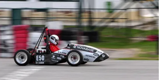
It is the team's second electric vehicle and the lightest prototype to date (Figure 1.2). The chassis is a carbon fiber reinforced polymer monocoque, the first monocoque used in a team prototype.
W ORK C ONTRIBUTION AND O BJECTIVE
The fifth prototype of the team, FST 05e, will be the test car in this work. This work aims to further develop the dynamic model of the vehicle to improve the vehicle dynamics understanding of the team and to assist in the design of the following prototypes.
D OCUMENT S TRUCTURE
In the third chapter, some definitions and concepts of vehicle dynamics will be presented to better understand the modeling of the vehicle as a system. Finally, in the seventh chapter, conclusions will be drawn and suggestions will be made for future developments of the model.
F ORMULA STUDENT EXPERIENCE
C OMPLIANCE M ODELING
In (Fischer 2001), BMW's contribution to the development of MSC ADAMS/Car is noted and the introduction of this environment in the company is also described. A similar context work to the above is also carried out in (Wale 2009), although to a lesser degree in complexity.
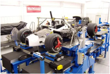
C OMPLIANCE M EASURING
The work covers, albeit in an iterative way, the process of designing, building and using the K&C test machine at the University of Aachen. In (Morse 2004) Phillip Morse (of Morse Measurements LLC) takes on the task of using K & C test data for practical use in suspension tuning.
F RAMEWORK
From the basic considerations in designing a K&C test machine to the process of running simulations and comparisons between computer-built models in MSC ADAMS and test data. This work is valuable because it shows more ways in which the test data can be used in addition to its already valuable contribution to vehicle modeling.
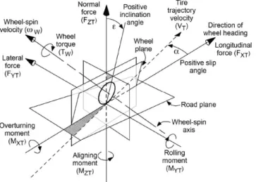
C OORDINATE S YSTEMS
The tire coordinate system is attached to the contact patch of each tire and guides the rotation of the wheel's z-axis. The rotations of the vehicle coordinate system relative to the ground coordinate system in x, y, and z are called the roll, pitch, and yaw angles.
S LIP P ARAMETERS
Sideslip angle
The purpose of this system is to represent the orientation of the wheels to calculate the forces developed by the tire (see Figure 3.3). The roll angle and x and y positions will be used to represent the vehicle's path in the XY plane.
Slip angle
11 The following two quantities of slip are important in tire dynamics and their influence on contact patch force generation will be explained later.
Longitudinal Slip Ratio
V EHICLE G ENERAL C HARACTERISTICS
Vehicle Dimensions
Vehicle mass properties
S USPENSION & S TEERING P ROPERTIES
Wheel Angles
The camber angle, γ, is the angle between the z-axis of the vehicle and the wheel surface measured around the x-axis of the vehicle. The convention is that it is positive when the top of the wheel leans towards the vehicle.
Steering axis & properties
15 An important control characteristic for the modeling approach for the control system is the c-factor of the control system. The definition of this characteristic for a linear control box is the rack displacement per rotation of the input shaft.
Instant Centers
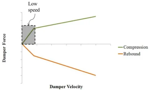
S USPENSION S PRINGS AND D AMPERS
Because the main purpose of the model is to give a hint about changes in vehicle performance, the normal cornering situations will be taken into account. In terms of roll behavior, some racing cars are usually equipped with anti-roll bars (ARB), which is the case with the FST 05e.
D RIVER I NPUTS
A description of the drivers' input will be done first, then the various subsystem models that separate the longitudinal dynamics and lateral dynamics of the vehicle for better organization will be presented.
T IRE M ODELING
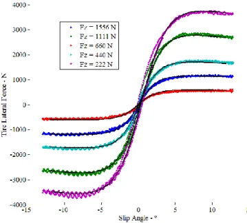
- Tire Lateral Force
- Tire Longitudinal Force
- Self-Aligning Torque
- Tire Model – Pacejka’s Magic Formula
- Tire Testing
- Model Fitting
This self-adjusting torque arises due to the lateral force distribution of the tire in the contact print. The tire lateral force fit under pure slip conditions (slip angle only) is shown below.

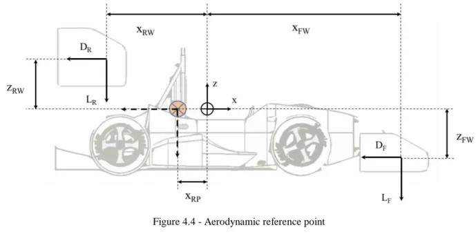
A ERODYNAMICS
With these coefficients it is possible to easily calculate the forces and moments present in the tire by determining the operating conditions. D and L are the drag and lift forces, and CD and CL are the drag and lift coefficients. This results in a point that has all drag and buoyancy forces and no moment.
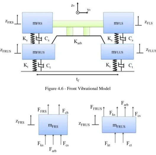
V EHICLE V IBRATIONAL M ODEL
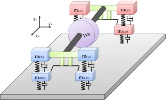
Model layout and components
Model formulation
As you can see, there are 9 independent DOFs in this system, the vertical displacement of each mass system and the roll of the chassis.
Mass, Stiffness, Damping Matrices and Force Vector
The same set of equations can be written for the rear of the vehicle. The direction of the forces in the formulas is as they act on the unsprung mass, which means that the same force acts on the sprung mass in the opposite direction. Equation (4.29) gives the change in the vertical load on each axis due to the longitudinal acceleration of the sprung mass.
D YNAMICS OF A PARTICLE IN NON - UNIFORM CIRCULAR MOTION
Since it is more common to use the accelerations and velocities in components of the vehicle coordinate axes. In this model, only planar motion with three degrees of freedom will be considered when defining the horizontal motion of the vehicle. For simplicity, the effect of the rotation around the vehicle's x and y axis will not be taken into account when defining the vehicle's motion.
V EHICLE L ONGITUDINAL D YNAMICS
Motor
The torque delivered to the transmission is then controlled by the throttle pedal percentage, P%, depressed by the driver. A vehicle's transmission is a gearbox with only one input-output ratio, this is called the transmission ratio, TR. Since the FST 05e has a motor and gearbox for each of the rear wheels, the above equations are used for both wheels.
Brake System
The force of the pedal is shared between the two master cylinders by a device called the balance bar (Figure 4.17). The purpose of this balance bar is to adjust the balance of braking force between front and rear to the specific wishes of the driver or engineer. The position of the balance bar and its orientation have also been chosen to give the driver a mechanical advantage.

Wheel rotational dynamics and force calculation
By calculating the angular acceleration of the wheel when subjected to the moments described above, the advantages of the Matlab Simulink environment of loop systems, differentiation and integration can once again be used. By differentiating the angular acceleration, the angular velocity of the wheel is obtained, which serves as input to the calculation of the longitudinal slip ratio, as described in Chapter 3.
V EHICLE L ATERAL D YNAMICS
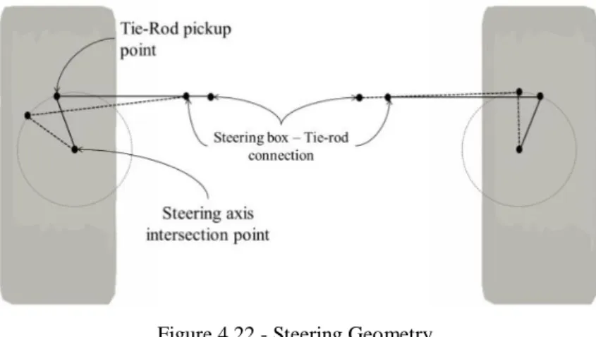
- Steering Mechanism
- Sideslip and slip angles calculation
- Inclination angle calculation
- Force and moment calculation
The solid lines represent the nominal position of the steering system with no wheels steered. The lean angle as defined in chapter three will be calculated using the displacement of the wheel and also the orientation of the wheel. Since the steering axis is not normally vertical, the steering of the wheel causes the angle of inclination to undergo changes according to said geometry.
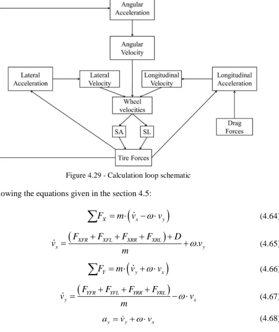
V EHICLE ACCELERATIONS
Tires and aerodynamic forces are needed to calculate the vehicle's longitudinal and lateral accelerations. To calculate the angular acceleration of the vehicle, it is necessary to calculate the moment of oscillation about the center of gravity of the vehicle. The longitudinal, lateral, and angular velocities can then be used in calculating the ratio of longitudinal slip to slip angle.
V EHICLE M OTION
It is also possible to describe the trajectory of the vehicle's wheels using the relative position of the wheels in relation to the vehicle's coordinate system. Using these positions, one can plot the trajectory of the vehicle's CG and its wheels in the XY plane.
S IMULATIONS
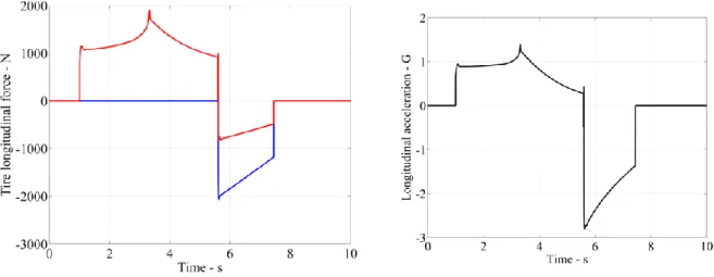
Straight line acceleration and braking
The purpose of this is to simulate the behavior of the vehicle in the acceleration event from the Formula Student competition and also to evaluate its braking performance (Figure 4.32). The vehicle then brakes without locking the wheels until it comes to a complete stop around the 7.5 second mark, see Figure 4.34. Figure 4.35 shows the development of aerodynamic and vertical tire loads during the simulation.
Skid Pad simulation
This effect is due to the vehicle's vector velocity being longitudinal at the moment the wheels are steered. In Figure 4.41, the yawing moment of the vehicle can be seen and steady-state is achieved to maintain a constant radius and turning speed. Below you can see the vehicle's center of gravity path to ensure that the vehicle is within the track boundaries (Figure 4.46).

P ARAMETERS WITH INFLUENCE ON VEHICLE BEHAVIOR
Vertical Load
Slip angle
Inclination angle
L OAD CASES CALCULATION
57 By introducing an extension of the contact patch to the upright body, the tire forces and moments can be easily introduced to extract the loads in each suspension link (Figure 5.3). This rigid body is constrained by the upright in all three directions, but also in two rotations, around the x-axis of the wheel and the steering axis. A band lateral force must be applied to the contact patch extension of the strut to reflect the reaction moment due to the rotational constraint about the x-axis of the wheel.

D EFORMATION ANALYSIS
Steering shaft
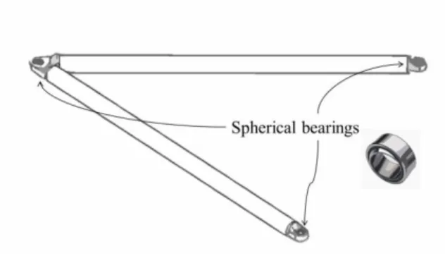
Wishbones, Tie-rods and Toe-rods
After obtaining the loads present at each connection, its deformation can be calculated using the elastic properties of the component. Where F is the force present in the link and Alink is the cross-sectional area of the suspension link. Using solid mechanics the shear stress and subsequent displacement of the bonded joint can be calculated (Figure 5.19).
M ODEL S CHEMATIC M ODIFICATIONS
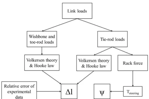
- Component loads calculation
- Deformation calculation
- Steering mechanism modifications
- IA calculation modifications
The joint activator uses the elongation of the connecting rods calculated in the deformation calculation subsystem to apply the displacement to the joint. In the compatible model, the equations are modified to use the elongation of the guide links in the three-point method routine (Figure 6.4). The correspondingly modified wheel yaw angle also enters the IA calculation, but is directly included in the calculations as in Chapter Four.
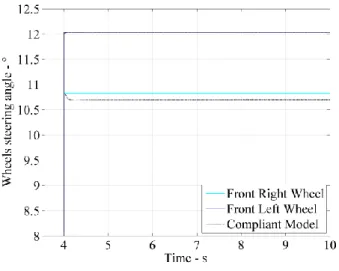
C OMPLIANT S KID P AD SIMULATION
This compliance causes the inclination angle of the wheels to change from the nominal values of the rigid simulation. The lateral forces at the tires underwent changes and from the obvious looking at the data above, the right front wheel was the one most affected. As one can see, the forces take a longer time to reach a similar value to that of the rigid model simulation and this is not related to the variables above because they roughly conserve the.
C ONCLUSIONS
Confirmation of the results with further physical testing, preferably with an instrumented FST 05e, would be beneficial and is certainly a missing piece of this work. In addition to this fact, this work can contribute to the next prototyping process for Projecto FST Novabase and serve as a foundation for further improvements of the vehicle dynamics simulation carried out by the team.
F UTURE D EVELOPMENTS
The equations have some minor simplifications and most scaling factors are set equal to one. To calculate the volume fraction of fiber and matrix in the layer, the following equation is used, where g symbolizes the weight per surface area of the fiber and the density is represented as ρfiber. To calculate the final laminate stiffness matrix, several stiffness matrices from several layers present must be collected.