In particular, the application of computer simulation has been crucial to the development of the field. The second term of the course will cover applications of simulation in a number of other areas, including operations analysis, insurance and finance. There is some overlap in these three, but in this course the focus is on the second and third of the above.
The first is to gain some understanding and knowledge of the techniques and tools available. The second is that many of the techniques themselves are smart applications or interpretations of probability and statistics. Here we will use the experiment to calculate an estimate of the needle length.
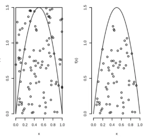
The reason for this is that if we let X be the distance from the center of the needle to the nearest bottom grid line, and Θ be the angle the needle makes with the horizontal plane, then assuming a random needle toss, we have X ∼ U[0, d] and Θ ∼U[0, π]. Namely, after d≤M steps, one of the numbers i/M will appear a second time and the algorithm will then produce repetitions of cycles of length d or less. To improve the efficiency of the procedure and allow for situations where f may be unbounded or have unbounded support, the technique can be modified to allow the boundary function to take the arbitrary form Kg(x), where g is the density of a distribution from which it is easy to simulate .
An adaptation of the rejection algorithm that works well for many distributions is the ratio of uniforms method. The point is that, in the ratio of uniforms method for example, the slowest part of the algorithm may be to check whether (u, v)∈ Ch or not. This variance can be very low, much lower than the variance of the estimator θˆ given in (6), if g can be chosen such that ψ is almost constant on the set {x∈R:g(x)>0}.
Markov chain Monte Carlo
The mean value cannot be determined explicitly, but as we will see, it can be found by simulation, using MCMC. The Metropolis-Hastings algorithm is a general algorithm that can be used to simulate from a density f of an m−dimensional random variable. At each step of the algorithm, a new 'candidate' value Y is proposed according to a proposal density q(y|Xt) which may depend on the actual state Xt of the Markov chain.
The density q(y|Xt) is replaced by the density q(v|Xt) of the template V. Under conditions of mild regularity, the Metropolis-Hastings algorithm will generate a Markov chain that has a distribution with density f as its equilibrium distribution. We will conclude this section by examining how the Metropolis-Hastings algorithm can be used to simulate the Strauss model. In this section, we will provide the basic concepts and results related to Markov chains that are necessary to prove that the Metropolis-Hastings algorithm actually works.
Let {Xt}∞t=0 be a Markov chain on Rm such that for any t the conditional distribution of Xt given X0,. The density f is called invariant for the Markov chain{Xt}∞t=0 if Xt has density f ⇒Xt+1 has density f. It can be shown that if {Xt}∞t=0 has the equilibrium distribution with density f, then f invariant.
Practically, every Markov chain Monte Carlo algorithm is constructed so that f becomes invariant. It can be shown that for a time homogeneous Markov chain with invariant density f the transition probabilities converge if the additional chain is uncrossable and aperiodic. It can be shown that (20) holds for almost all x and all A ∈ B(Rm) if the chain is uncrossable and periodic and has f as an invariant density.
In this section, we will show that by choosing the acceptance probability as described in Algorithm 6, the resulting Markov chain becomes reversible, i.e., as in Section 2.6, the goal of MCMC simulations is usually to evaluate an integral of the form If the Markov chain {Xt}∞t=0 is estimated to be in equilibrium at time t0, then θ is estimated by.
More specifically, (28) holds if Eϕ(X)2 <∞ and the Markov chain {Xt}∞t=0 is a so-called geometric ergodic. This is especially used in contexts where the density f is of the form
Models for point processes
By using the definition of a Poisson point process, it is possible to derive a formula for probabilities associated with the Poisson point process. Note that if we let g be the indicator function of the event F, we again get (32). In this section we will define and study Markov point processes. These are finite point processes with a very simple interaction structure.
The requirement (M2) in the definition is the essential one, which relates to 'the conditional intensity of adding an extra point u to the point pattern x'. A point process X with density f is a Markov point process with respect to the relation ∼ if for all x∈ S. the Poisson point process). This process is Markov with respect to any relation ∼ since f(x)>0 for all x∈ S and λ(u;x) =λ is constant for all u and x such that u /∈x. Hard-core model) Suppose we want to model a pattern of non-overlapping circular disks of fixed diameter R >0.
The density of a Markov point process can be factorized in a simple way as described in the famous Hammersley-Clifford theorem. The set of cliques is denoted C. The Hammersley-Clifford theorem gives a factorization of the Markov density in terms of interactions that are allowed only between elements in the clique. Hammersley-Clifford)A density f defines a Markov point process with respect to ∼if and only if there exists a function ϕ :S →[0,∞) such that ϕ(x) = 1, unless x∈ C and such that.
We are not going to prove the theorem here, but just mention that a long but rather elementary proof can be constructed, based on induction. The Hammersley-Clifford theorem is important, first, because it provides a way to break up a high-dimensional joint distribution into manageable clique interactions that are easier to interpret and have a lower dimension. If we condition on the number of points in x, we get the Strauss model described in Part 1, Section 3.1.
The area interaction process) In this example, we consider an alternative to the Strauss process called the area interaction process. From the actual shape of the conditional intensity, we can deduce the shape of the corresponding density.