A proof of Luttinger's theorem

Dans ce cas, la surface de Fermi est la surface où, dans l'espace des moments, le nombre moyen de i. Selon le théorème de Luttinger, le volume contenu dans la surface de Fermi d'un système de fermions en interaction ne dépend pas de l'interaction.

Interacting Electrons in a Weak Magnetic Field 113

FIELD THEORY FOR MANY-FERMION SYSTEMS 3

In the mathematical analysis of the problem, we start directly with the mutual dispersion relation e(p) and not with the band function. The anti-term is then chosen so that the Fermi surface defined by the zero set e(p) remains invariant.

FIELD THEORY FOR MANY-FERMION SYSTEMS 5

The occupation number

Luttinger's Theorem

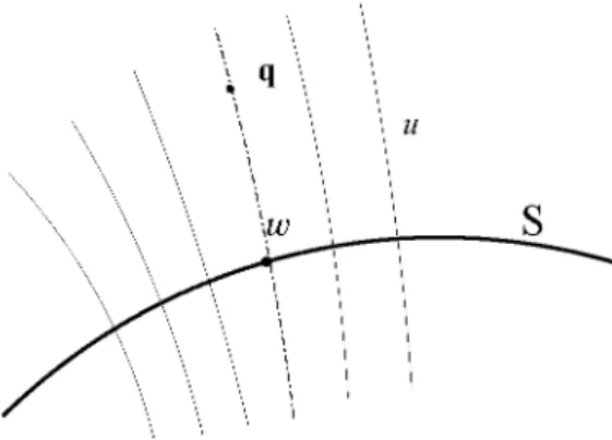
The physical (or interacting) Fermi surface Sß of the system is the

Sketch of the Proof of p(X) = p(0

The Thermodynamic Limit
The Renormalization
Scale Decomposition

Spin Magnetization
SPIN MAGNETIZATION 11
THE ASSUMPTIONS 15
THE THERMODYNAMICS 17
THE THERMODYNAMICS 19

Green's functions on finite lattice, and their convergence to Green's functions of. Then the sum of the volumes enclosed in the Fermi surfaces is independent of .

QW,AQW)

GREEN FUNCTIONS 21

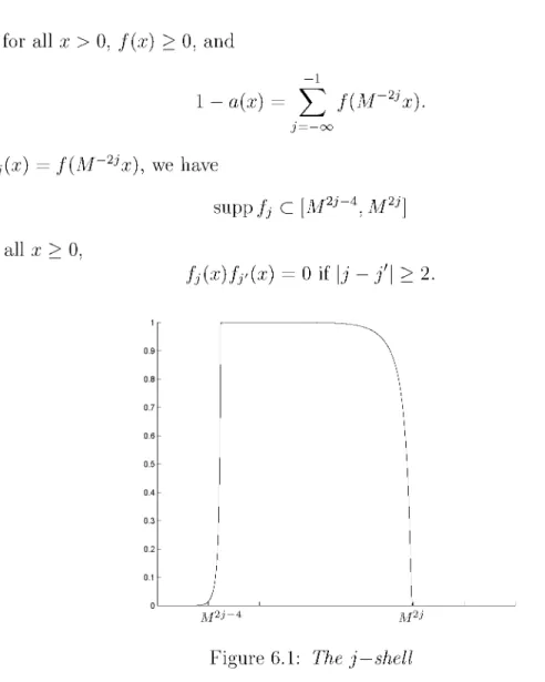
In a first step, the propagator is regulated by an infrared cutoff at energy scale M1 with / < 0 and M > 1. As long as this cutoff is present, the regulated Green functions G2m are analytical in the thermodynamic limit.

THE INFINITE VOLUME LIMIT 23

I(p) = (l-GI(p)CI(p))-lGI(p),

KI(V) = Y^KIÀV)

The density of Fermions in the infinite volume, defined by the formal

THE INFINITE VOLUME LIMIT 25

The density of fermions p^L> (A) converges in the sense of formal power series to. Then the density of fermions in the thermodynamic limit is independent of the interaction, that is, formally.

CONTRACTIONS AND NORMS 29

To prove the analyticity of the model on the finite grid, we use the following.

BOUNDS FOR THE COVARIANCE 31

Here: • : denotes the Wickian order with respect to the covariance of C. ii) Define the covariance of C on B x B as follows:. v) The covariances Cu(ß, £') and Cs(ß, £') are defined in the same way as the covariance.

A~' Using

BOUNDS FOR THE COVARIANCE 33

BOUNDS FOR THE COVARIANCE 35

The Analyticity of the Green Functions

THE ANALYTICITY OF THE GREEN FUNCTIONS 37

For the four-point function, .. ii) The connected two-point Green function S2 (x,y) is analytic in A with.

THE ANALYTICITY OF THE GREEN FUNCTIONS 39

The Projection onto the Fermi Surface

The sum over A^ and over {], {} is finite, such that the number of the voice is well defined. The sum over AL is also finite, so the density is well-defined and analytic. As we saw in the last chapter, Green's functions on a finite lattice are analytic, with

Furthermore, it turns out that the green functions diverge with each order in A while L tends to infinity. Here Via is the derivative of the grid defined above with respect to the a component of the ith variable. On the finite lattice AL we need a localization operator β^ that maps points of the lattice onto other points of the lattice.

For the projection / on the Fermi surface we give here the main results of [7], and refer.

THE LOCALIZATION OPERATOR 43

Let (p, lo) denote the coordinates defined in the previous lemma. p, lo) denotes the coordinates defined in the previous lemma.

Figure 4.1: The projection onto the Fermi surface

THE LOCALIZATION OPERATOR 45

The Projection on the Lattice

Suppose Vk for every point k G AL is the fundamental cell of the lattice containing k.

Figure 4.2. The lattice and its fundamental zone

THE LOCALIZATION OPERATOR 47

THE LOCALIZATION OPERATOR 49

By hypothesis k G Ug(S), and x(k) = 1- Since the projection is constant with respect to fco, we consider only the derivative with respect to the spatial variables,.

THE RENORMALIZATION CONDITION 51

THE RENORMALIZATION CONDITION 53

For |A| < A0,

For dispersion relations eßL^ defined in 2.10, there is a unique countert¬

THE RENORMALIZATION CONDITION 55
THE CONVERGENCE IN THERMODYNAMIC LIMIT 59
The Convergence in Thermodynamic Limit

The sequence of the u^ is thus a Cauchy sequence in the Banach space of functions on AL x C that are analytic in A. For the two-point (non-amputee) Green function, .. ii) The counterterm Kr on order r in A is defined in the same way:. We define L(G) as the set of internal lines of GJ and E(GJ) as the set of external lines.

It follows that the two-sided vertex Kr cannot enter the composition of the second term. We obtain an inductive procedure for determining the order of antiterms .. in order in A given by .. the right-hand side containing only antiterms of order r' < r in A. 5.2 Convergence in the thermodynamic limit. For each L E N there exist constants A0, B0 and Bx which are independent of L but dependent on r such that .. iii).

In thermodynamic limit, the density p(LßX) converges in the sense of formal power series to p(X), that is for all r > 0,

SCALE DECOMPOSITION 63
fßk2 + e2(k))

THE TREE EXPANSION 69

In this section we prove the convergence of the Green functions in thermodynamic limit .. at every order in A. The proof given here follows the proof given in [7] on the continuum . momentum space, which performs the same scaling decomposition and uses the same force. The effective cutoff implement in definition 2.10 allows applying the same bound as in . the ongoing matter. The problem of calculating a possibly divergent integral is replaced by.. the question of the convergence of series.

To perform the decomposition over the scales, we first define a G°° partition of the unit. .. ii) The propagator on scale j < 0 of the model in the infinite volume is determined by . iii). Let G G S2m(r) be one of the connected, amputated graphs that contribute to G2Jir. decompose all propagators of the graph G using the scale decomposition. Uf is the number of upward branches of the fork lL(Gf). then the number of legs of / in t. iii) The rootß of the tree t(GJ) is the fork corresponding to the graph GJ.

We call "two-legged leaves" the leaves corresponding to two-legged vertices of GJ, and "four-legged leaves" the leaves corresponding to four-legged vertices of GJ. v) The graph G(f) is obtained by folding all subgraphs Gg with nβj) = f.

It is possible to show (See [7] and [6]) that the sum over the graphs of

THE TREE EXPANSION 71
THE POWER COUNTING 73
THE IPI GRAPHS 79

Non-Overlapping two-legged Graphs

Note that the degree of the fork / is independent of the root degree of GJ. By following this procedure, all two-legged leaves of the t(GJ) graph can be replaced by c-forks, ending up with a new t-tree that has only four-legged leaves. The value of the graph G associated with the root of / must be calculated inductively, first substituting it. in G any subgraph G/ connected by a c—fork / from a vertex with vertex function.

The . sum also runs over the labeling of the two-legged forks in s, r, and c forks. The contribution of an IPI, two-legged fork / to the value of the graph is given by. The momentum in G(ß) can be set so that each line of the spanning tree carries an external momentum.

If the root scale j of GJ is strictly negative, L(GJ) decomposes into the set of lines of G((f)), which is on scale j, and the set of lines of subgraphs corresponding to forks in .

Let G be a connected, two-legged graph with A vertices, all having

Let G be a connected, two-legged graph, all vertices of G having even

THE IPI GRAPHS 81

The Graph G'

G' has only two-leg and four-leg vertices with vertex functions that are either interaction vertices or IPI values of two- or four-leg subgraphs of G. The only non-trivial two-leg subgraphs of G' are the sets of soft two-leg vertices of G' and every non-trivial four-leg subgraph of G' consists of a single quadruped. A graph G corresponding to a tree t is obtained by collapsing all two- or four-branched subgraphs of G into nodes, t has no split corresponding to a non-trivial two- or four-branched subdiagram, but it is not a tree with the given properties because the leaves need not t correspond to the IPI subgraphs of G.

The . external legs of Gf are of scale j^/) or higher, and according to the support property of the propagators, the scales of the propagators of the string are in {j^f),Jtt(/)+1} - Therefore, Gf ' n string of two-leg graphs, connected by propagators on scale jf = jx{f) + 1- The vertex function corresponding to / is given by. The case where Qt corresponds to an s-fork is treated in the same way as the same. If / is quadrilateral and one particle is reducible, remove the strings attached to Gf. and adds a leaf above the fork / for the IPI kernel of Gf, as well as for each IPI 2-leg subdiagram Qt of the strings.

If jw = 1, then w is also a vertex of G, and the associated function is v. Otherwise, jw is the root scale of a subgraph of G, whose value is a vertex function in G', and jw is summed.

By construction, all the two-legged vertices of G' have label r or c, but not s, since the last would correspond to one particle reducible graphs

THE IPI GRAPHS 83

Bounding the Value of IPI Graphs

THE IPI GRAPHS 85

Proof: This theorem is proved by induction on the depth of the pair (t,G), that is.

THE IPI GRAPHS 87
REMOVING THE CUTOFF 89

Lemma 4.15 can be applied to the support properties of the propagator in scale Jtt(w) accompanying Fw. If w corresponds to the same scale insertion, then there is no sum over the scale jt We therefore get. IfFw belongs to a four-legged vertex and Gw is non-overlapping on the scale jw.

Removing the Cutoff

The Convergence of IPI Graphs with j fixed

where B is Co, Ci or L

By hypothesis, the first term on the right-hand side tends to zero when L -=> oo. Let Zi(Z_, B) be the space of absolute additive sequences in the Banach space. ii) Let G be an IPI graph with 2m external legs and let f be a planar tree rooted at ß compatible with G such that the pair (G, t) contributes to the renormalized Green's function G2ßir or G2mr on scale j < 0. By the same argument as for the c—fork, we see that in the sup-norm,.

Since they are no sum, and no projection operator ßL\, the convergence is given by .. w corresponds to a four-legged forks. Since the sum over the root scale jw is at most \j | has terms, and that Fw contains .. no projection operator ßL\ the convergence follows from the LH. We now turn to the proof of the claim for G', by the fact that G' is a graph with . vertex functions F^ or Fw converging to Fw in the limit / — —oo resp.. value of G' is given by the integral of a bounded function with compact supports.. convergence in L follows in the same way.. i ) Let G be an IPI, two-legged graph, contributing to the self-energy at order r in A, and t a tree compatible with G rooted at ß.

The highest norm of the two-point Green function is bounded in the same way.

Let G be a IPI, two-legged graph, contributing to the self-energy Er,

The Convergence of G22r in *ne ^i—norm
l Integral Bound

SYMMETRIES 105
SYMMETRÎES 107
SYMMETRÎES 109
ÎNTERACTÎNG ELECTRONS ÎN A WEAK MAGNETÎC FÎELD 113
Interacting Electrons in a Weak Magnetic Field
Luttinger's Theorem
EXAMPLE: SPHERÎCAL FERMÎ SURFACES 117
Example: Spherical Fermi Surfaces
EXAMPLE: SPHERÎCAL FERMÎ SURFACES 119

Salmhofer, Renormalization: An Introduction, Springer (1999)

The sum over the scale of the four products over the forks is bounded by. The Grassman Gauss integral with covariance G is then the unique linear map on the space of the Grassman functions. Proof: Without loss of generality, we can assume that the vectors f% are linearly independent.

Corollary B.12: The generating function for Green's functions is invariant under the symmetries of the Hamiltonian. 2 To avoid confusion with fiß, we use Ep for the Fermi energy, instead of the usual /x notation for the chemical potential. IR x T in the (formal) Green function Ga of the model in the infinite volume with.

Then the sum of the volumes enclosed by the Fermi surfaces is independent of . Let us consider a system of fermions, described by the band function ea(k) = ^. l)apBh, where mig and pB are the mass of the fermions and the magnetic moment. The case of a spherical Fermi surface is thus special in the sense that the volume of each Fermi surface is independent of the interaction strength.