The linear fractional stable motion (LFSM for short) is the focus of this thesis. Special attention is paid to our implementation of the FFT-based simulation method developed by Stoev and Taqqu [40].
Introduction to mathematical tools
In this work, special attention is paid to the subclass of L´evy processes – stable processes. It is fully characterized by the scaling parameter σ > 0, the self-similarity parameter H ∈ (0,1) and the stability index α ∈(0,2) of the driving stable motion.
Introduction
This is a consequence of the work of Pipira and Taqqu [30], which in turn applies the decomposition results from the seminal work of Rosinski [36] (see also [38]). In this paper we will propose a new estimation procedure for the parameter θ = (σ, α, H) in the high and low frequency framework.
First properties and some asymptotic results
Given the self-similarity of the process (Xt)t∈R, we can easily find that (nH∆n,ri,kX)i≥rk d. The strong law of large numbers in Theorem 2.3.1(i) will be useful to estimate the parameter H .
As we indicated above, in the framework of pure jump α-stable drift motionL, the central limit theorem never holds ifk= 1. Since the parameter Hent the quantity ϕhigh(t;H, k)n via nH, the additional term (logn)−1 appears in the convergence rate.
Statistical inference in the general case
According to Theorem 2.3.2, we are in the domain of validity of a central limit theorem when H <1−1/α, while a non-central limit theorem holds if H >1−1/α. The next theorem presents the statistical behavior of the estimator (σelow,αelow,Hblow(−p,bklow)n) in the case α−1∈N.
A simulation study
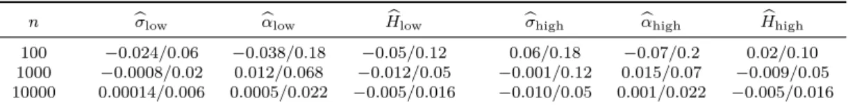
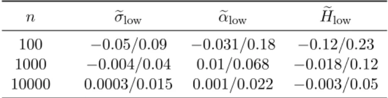
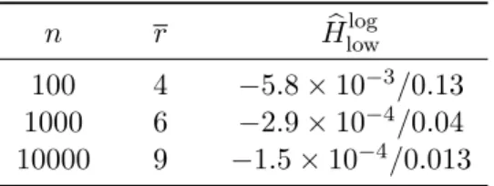
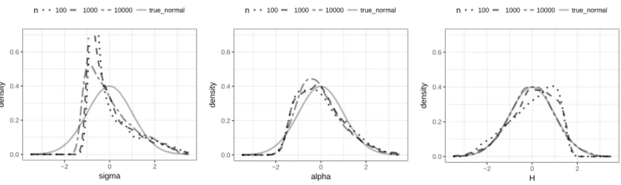
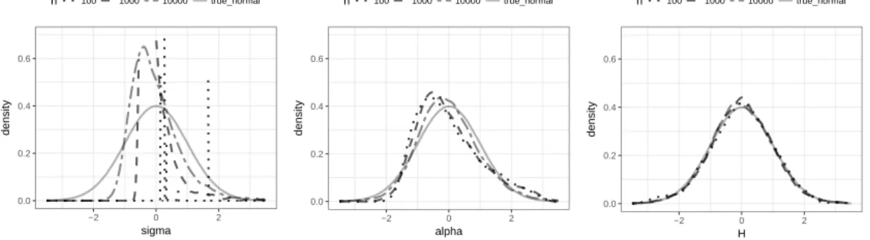
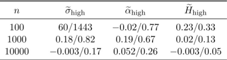
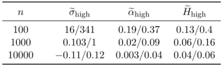
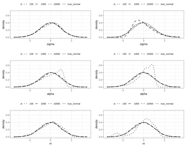
The next table shows the final sample bias/standard deviation of the estimator Hblowlog in the setting of Theorem 2.4.1 with p= 0.4,k=2 and r=blog(n)c. On the other hand, alpha estimator is not as sensitive to error due to the double logarithm. Furthermore, it is well known that low values of the parameter provide more efficient estimators in the setting of a fractional Brownian motion.
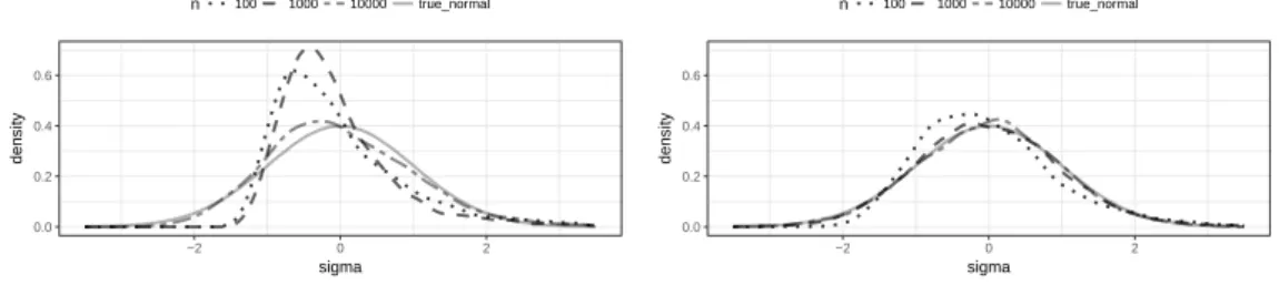
We also observe that the estimator of the parameter σ exhibits the worst finite sampling properties in the neighborhood (σ, α, H. Finally, let us discuss the finite sampling performance of the high-frequency estimators from Theorem 2.5.5. We observe that the estimators of the parameter σ has the worst performance and we only obtain reasonable results for n= 10,000.
The poor performance of the estimator of σ in Theorem 2.5.5 is explained by the fact that not only do we need a preliminary estimation step for our procedure, but we also first have to estimate the parameters H and α to arrive at an estimator of σ to obtain. We see a much better finite-sample performance, confirming that the poor finite-sample properties of the estimator of σ are largely due to a preliminary estimate of (α, H).
Proofs
Here we will show some technical results which are necessary to prove the main theorems. Note that, similar to (2.3.4), the latter connects power functions with characteristic functions which are explicit in the α-stable case. To prove the first part of the statement, we will use the inequalities in Lemma2.7.3.
The main ideas come from the work [7] and we will adapt their principles to our environment. In this case it is a consequence of the fact that it is a bounded and even function. Z(1)whereZ(1) is ad1-dimensional centered normal distribution and assumes that each coordinate Y1,j(2), 1 ≤ j ≤ d2, is in the domain of attraction of a β-stable random variables, i.e.
Thus, applying Theorem 2.3.2 and Proposition 2.5.2 and using the same arguments as in the proof of Theorem 2.4.1, we conclude the convergence. The results of Theorem 2.5.6 follow the same methods as presented in the proof of Theorem 2.5.3.
Appendix
Stepan Mazur specifically to study numerical properties of estimators related to stable piecewise linear motion. It is open source software licensed under the GPL-3 and is available on CRAN, the Comprehensive R Repository Network [1], which is today's largest repository for controlled R packages. There is a gitlab developer repository [2 ] for this project, where you can find the latest version of this software, as well as all the codes for the numerical experiments we have performed regarding LFSMs.
I would like to mention the contribution of Mark Podolskij, whose intuition and experience guided me and Stepan during the early stage of developing and debugging the package, as well as that of my colleague Mathias Ljungdahl, who pointed out issues of important performance and brought a new estimator to the package. In Section 3.3 we present the simulation method for lfsm sample paths and its implementation in our path function. Next, we present functions for finite sample studies of statistical estimators and some other functions.
Section 3.4 describes the implementations of the high- and low-frequency parameter estimators and discusses the reasons for their numerical behavior. Finally, in Section 3.5, we propose an object-oriented system that simplifies the software programming of L´evy-driven integrals.
Introduction
Basic R functions
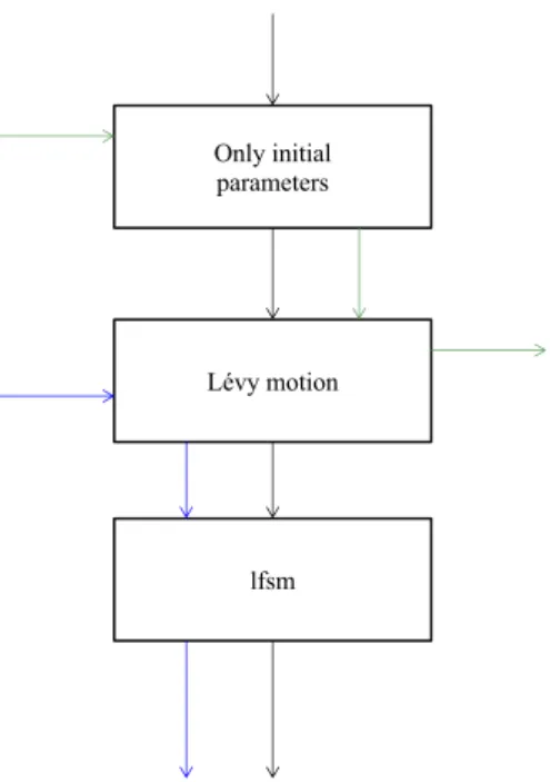
Green arrows: when L´evy motion without lfsm is needed to save processing time, the algorithm bypasses the later calculation. The path function returns a list containing the lfsm, the underlying L´evy motion, the point number of the motions from 0 to N (point_number) and the corresponding coordinate that depends on the frequency, the parameters (σ, α, H ) which was used to generate the lfsm, and the preset frequency. We recall that direct calculation of the sum approximating the integral in the definition of lfsm (3.2.1) would involve number of operations proportional to N M m, which makes the method slow.
Further, steps indexed [0;mN−1] are cut and fixed at the end so that the actual tail of the L´evy driver is at the beginning. In the first example, we study the GenLowEstimestimator and its bias and variance dependence on the length of the sample paths. Once done, CLT continues to the next length value until it reaches the end of the vector of lengths.
In this section, we describe aspects of some of the other features implemented in the package. Evaluation of the increments on a sample path of length N requires (k+ 1)(N−kr) operations-k+ 1 sums for N −kr points.
Parameter Estimation of the linear fractional stable motion
Now, we consider stable estimators for the self-similarity parameter H in the high and low frequency setting, defined by . The estimators for the stability index α of the steady-state motion in the high- and low-frequency setting are based on the empirical characteristic functions given by. The estimators for the scale parameters σ at high and low frequency are also based on the empirical characteristic functions which are determined for a value of t > 0.
Since we do not know ifαb0low(t1, t2)nis in the attraction field, we determine the estimator of the parameter kas. In the second step, we use the estimator ˆklow := ˆklow(t1, t2)n to estimate the parameters H,α and σ. Next, we consider the two-stage estimation procedure in the general case in the high-frequency setting, which is the same as in the low-frequency setting.
We illustrate this effect with the following experiment, in which the common high- and low-frequency estimators are compared with the corresponding continuous estimators. As a result, in cases where statistics bklow(1,2)n can be computed without encountering numerical errors, the performance of GenLowEstim and low-frequency ContinEstim is the same.

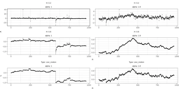
S4 classes for Levy-driven motions
Frequency indicator and indicator of process type are included in the class name, while motion, coordinates, parameters for which the path is simulated and the L´evy motion are written in the slots. Indicators of frequency and a process type are included in the name of a class, which is supposed to make a method dispatch more simple, without additional condition blocks. Parameters H, α, σ, as well as L´evy motion, coordinates and the lfsm itself are written in corresponding slots.
In the following example, we see how an instance of classSimulatedLfsmLowis is created and then plotting and inference are performed using generic functions plot and ContinInfer. In this example, the plot function requires almost no effort compared to the equivalent from Section 3.3, which is because a generic plot method and objectSimulatedLfsmLow are defined. You can see that the plot (and, less clearly, ContinInfer) used 'Low' from the name of the class to perform calculations.
The authors acknowledge the financial support from the project "Ambit fields: probabilistic probabilistic and statistical inference" funded by Villum Fonden. Stepan Mazur acknowledges financial support from internal research grants at ¨Orebro University, and from the project "Models for macroeconomics and finance after the financial crisis" (Dnr: P18-0201) funded by the Jan Wallander and Tom Hedelius Foundation.

Appendix
In this chapter we will discuss methods for simulating a certain type of stochastic integrals. We are interested in kernel functions with two specific characteristics - singularity near zero and a long tail at infinity. We propose to use a combination of two different methods to calculate integrals of the type (4.1.1): the one developed by Cohen et al.
17] must be used near singularity points, and the method based on the convolution theorem - outside this area. The idea to mix several techniques while computing a stochastic integral comes from previous papers by Bennedsen et al. In this chapter we consider L´evy drivers, although we note that the technique based on the convolution theorem allows more general random measures and even different types of integrals.
Shot-noise approximation of non-Gaussian fractional fields
Review of the multidimensional discrete Fourier transform 77When ν(R) =∞, the integral (4.1.1) is approximated by a superposition of a shot noise.
Review of the multidimensional discrete Fourier transform
Algorithms based on multidimensional fast Fourier transforms
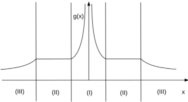
To capture two features of the kernel, described in Section 4.1, we propose dividing the kernel domain into three pieces, subsequently computing (4.1.1) separately on the first two, and truncating the third, Figure 4.1.
This property prohibits the use of the error bound for long decreasing tails of kernels because smaller values of the function will be assigned the same error bounds. Scaling properties of the empirical structure function of linear fractional steady motion and estimation of its parameters. Kinetic equation of linear fractional steady motion and applications to modeling the scaling of intermittent eruptions.