Bounded Love of Variety and Patterns of Trade - CiteSeerX

2009-10

Sw is s Na ti on al B an k W or ki ng P ap er s

Bounded Love of Variety and Patterns of Trade

Philip Sauré

The views expressed in this paper are those of the author(s) and do not necessarily represent those of the Swiss National Bank. Working Papers describe research in progress. Their aim is to elicit comments and to further debate.

Copyright ©

The Swiss National Bank (SNB) respects all third-party rights, in particular rights relating to works protected by copyright (information or data, wordings and depictions, to the extent that these are of an individual character).

SNB publications containing a reference to a copyright (© Swiss National Bank/SNB, Zurich/year, or similar) may, under copyright law, only be used (reproduced, used via the internet, etc.) for non-commercial purposes and provided that the source is mentioned. Their use for commercial purposes is only permitted with the prior express consent of the SNB.

General information and data published without reference to a copyright may be used without mentioning the source.

To the extent that the information and data clearly derive from outside sources, the users of such information and data are obliged to respect any existing copyrights and to obtain the right of use from the relevant outside source themselves.

Limitation of liability

The SNB accepts no responsibility for any information it provides. Under no circumstances will it accept any liability for losses or damage which may result from the use of such information. This limitation of liability applies, in particular, to the topicality, accuracy, validity and availability of the information.

ISSN 1660-7716 (printed version)

Bounded Love of Variety and Patterns of Trade

Philip Sauré^†

Swiss National Bank

November 9, 2009

Abstract

Recent trade data exhibit the following four empirical regularities: (i) countries import only a small fraction of all traded varieties (ii) per capita income and the num- ber of imported varieties correlate positively (iii) per capita income and trade shares correlate positively and,nally, (iv) world trade shares have increased substantially.

The present paper argues that standard theories fail to explain at least some of these patterns and subsequently shows that a small and reasonable change in the demand structure can reconcile the New Trade model with the data. Its key assumption im- poses an upper bound on consumers’ marginal utility from varieties. This implies that consumers purchase only the cheaper share of varieties, while expensive foreign varieties bearing high transport costs are not consumed. Technological progress that increases per capita consumption of those varieties in the consumption basket de- creases marginal utility derived from them and induces consumers to extend their consumption to more expensive varieties produced at distant locations. Through this additional margin trade shares increase as productivity grows. Productivity growth is thus identied as a joint determinant of trade shares, the number imported varieties, and per capita income.

Keywords: Marginal Utility, Variety.

JEL Classications: F10, F13.

WI would like to thank Raphael Auer, Giancarlo Corsetti, Gino Gancia, Omar Licandro, Marco Maezzoli, Diego Puga, Morten Ravn, Karl Schlag, Jaume Ventura, Joachim Voth and an anonymous referee for many valuable comments. All remaining errors are mine.

†Swiss National Bank, Börsenstrasse 15, 8048 Zurich, Switzerland. E-mail: [email protected] The views expressed in this paper are the author’s and do not necessarily represent those of the Swiss National Bank.

1 Introduction

Recent trade data exhibit the following four empirical regularities: (i) countries import only a small fraction of all traded varieties (ii) per capita income and the number of imported varieties correlate positively (iii) per capita income and trade shares correlate positively and,nally, (iv) world trade shares have increased substantially. These patterns are both, well known and well studied. Yet, existing explanations typically rely on intricate models to address one of the patterns, while falling short on at least one of the others.

The present paper does not pretend to be the rst in addressing the four stylized facts.

Instead, its contribution is to show that they emerge naturally within the most basic model with trade in varieties — the Krugman (1980) model — under a small and reasonable modication of consumers’ demand structure.

As its key deviation from the standard framework, the present paper imposes that marginal utility be bounded. More precisely, as consumption levels of any given variety drop to zero, marginal utility of its consumption stays nite — instead of approaching innity as under standard preferences. This twist in the demand structure implies that consumers buy only the cheaper fraction of varieties and exclude the relatively expensive ones —i.e., the foreign varieties that are subject to heavy trade costs — from their consumption basket.

Consequently, bilateral trade relations can be zero (pattern (i)). Further, an increase in per capita income, brought about by a decrease of marginal production cost, increases consumption levels of varieties in the consumption basket and marginal utility derived from each of them falls. The varieties outside the consumption basket — the expensive foreign ones — become relatively more attractive. Thus, richer consumers include new foreign varieties in their consumption basket and thereby increase their expenditure share on imports. This jointly explains patters (ii) and (iii). Finally, the positive eect of per capita income growth on world trade shares contributes to explaining the overall growth in world trade shares — pattern (iv).

The above-mentioned empirical regularities mentioned have not gone unnoticed in trade literature. Dening varieties as goods dierentiated by production origin¹, Haveman and Hummels (1999) observe that most importers purchase a very small fraction of the vari- eties available, concluding that the "complete specialization model considerably overstates the extent of specialization [...] or the degree to which consumers value varieties." Help- man et al (2008) show that a framework of heterogeneousrms andxed cost of exporting à la Melitz (2003) generate zero trade ows whenxed costs of exporting exceed potential operating prots in export markets. The authors then successfully estimate their predic- tions, in particular the probabilities of positive bilateral trade ows for a given country

1This is a common denition ofvariety, which departs form the earlier denition by Krugman (1980) identifying a variety by therm that produces it.

-3-2-1012No. Varieties

-2 -1 0 1 2

p. cap. GDP Log Changes 1970-2000

Number of Varieties and GDP per Capita

-2-1012No. Varieties p. Good

-2 -1 0 1 2

p. cap. GDP Log Changes 1970-2000

Av. No. of Varieties per Good and GDP per Capita

Data Source: Feenstra et al (2005) and PWT6.2

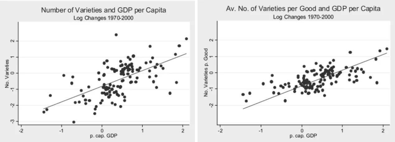
Figure 1: Postitve Correlation between growth in Number of Imported Varieties and per Capita Income. (Log-changes 1970-2000).

pair. While making signicant progress in this dimension, however, their model, by rely- ing on homothetic preferences, cannot account for the relation of per capita income and trade shares once total GDP is controlled for (patterns (ii) and (iii)).

Pattern (ii) is the least-known of the empirical regularities. Broda and Weinstein (2004) and (2006) document that from 1970 to 2000 importers generally increased the num- ber of source countries per good. In a related paper Schott (2003) reports that the US

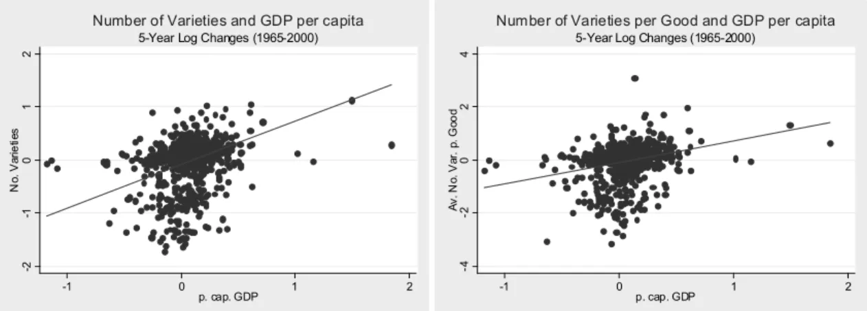
"increasingly sources the same products from high- and low-wage countries," which the author attributes to specialization within product categories. Figures 1 and 2 show that the changes in the number of imported varieties strongly correlate with changes in the importer’s per capita income. Dening a variety by 4-digit SITC good category and its ex- porting country, the left panel of Figure 1 shows that within a sample of 129 countries the Log-changes of the importer’s per capita income correlates positively with Log-changes in the total number of imported varieties; the right panel establishes a very similar relation between the importer’s per capita income and the average number of imported varieties per good². Figure 2 illustrates that the correlation of respective Log-changes hold also of ve-year intervals between 1965 and 2000³.

The third observation, the positive correlation between per capita income and trade shares, is well known but widely neglected. Empirical estimations of the well-known gravity equa- tion nd positive eects of per capita income and trade ows.⁴ Indeed, Anderson (1979)

2A simple OLS regression of Log-changes in the number of varieties (per good) on the Log-changes of importer’s GDP per capita renders estimated coe!cients of 0.97 (0.6) with t-statistics for the exogenous variable of 8.51 (9.33) and adjusted R-sq. of 0.36 (0.4). Controlling for changes in importer’s total GDP does not change signs and signicance levels. Importantly, total GDP is insignicant,i.e. that market size has little additional explanatory power. See the Appendix for a list of countries.

3The splitting into sub-periods decreases thet of the data but increases the relevant t-statistics.

4Hufbauer (1970) provides an early, Francois and Kaplan (1996) more recent empirical study. See also

-2-1012No. Varieties

-1 0 1 2

p. cap. GDP 5-Year Log Changes (1965-2000) Number of Varieties and GDP per capita

-4-2024Av. No. Var. p. Good

-1 0 1 2

p. cap. GDP 5-Year Log Changes (1965-2000)

Number of Varieties per Good and GDP per capita

Data Source: Feenstra et al (2005) and PWT6.2

Figure 2: Postitve Correlation between growth in Number of Imported Varieties and per Capita Income (Log-changes of 5-year intervals 1965-2000).

opens his seminal contribution with a specication that accounts for a non-trivial impact of per capita income on trade ows, admitting that, contrary to his model’s predictions,

“[t]rade shares ’should’ increase with income per capita.” The high tractability and the resulting analytical elegance of homothetic demand, however, make trade economists usu- ally opt for corresponding preference structures, preventing an independent role of per capita income in the gravity framework once total GDP is controlled for.⁵

The fourth and last of the patterns, the substantial rise in world trade shares, has been intensively studies in recent years. After Krugman’s (1995) account of the surprisingly divergent views concerning its causes, Baier and Bergstrand (2001) singled out tari re- ductions as its most important determinant. Yi (2003) subsequently argued that the observed increases in world trade shares imply excessive import elasticities in standard trade models (see also Bergoeing et al (2004) on this point). Substantial progress was made in explaining this "elasticity puzzle" as it was later labeled. Yi (2003) argues that increasing international vertical specialization caused the surge in trade volumes by making intermediate good enter trade statistics more than once, thus multiplying trade accounts. Ruhl (2005) puts forward that xed costs of exporting let more rms enter in reaction to permanent tari reductions than to transitory exchange rate blips and that this dierence accounts for the “elasticity puzzle”. Cuñat and Maezzoli (2006)), nally, show that reductions in trade costs can lead to diverging factor endowments, which adds an amplifying dynamic eect to the well-known static one, thus increasing the impact of tarireductions under common import elasticities. Yet, by relying on homothetic demand non of these studies accounts for the role of per capita GDP.

Ventura (2006) on the correlation between trade volumes and per capita income.

5Empirical studies investigating the impact of trade on growth generally control for causal links form income growth to trade openness through various instrumentation techniques (see Frankel and Romer (1999) or Alcalá and Ciccone (2004). Theoretical literature on this point, however, is much less developed.

The current paper adds to these literatures by providing a simple framework that oers a demand-driven explanation of the above-mentioned four empirical regularities. In order to quantitatively evaluate the extend to which it can explain the empirical patterns, the model is calibrated to match the US import shares between 1972 and 2000. This simple exercise shows that, with US tari reductions, income and population growth from the data the model matches observed US trade shares at a import elasticity that averages around 3.7 (it peaks at an 8.8 in 1972 and is lowest in 2000 with a values of 1.7).

This elasticity is still on the high side of estimates empirical estimates but constitutes substantial progress. At the same time, the model does replicates fairly well the increase in the number of varieties per good. As about half of the observed increase in trade volumes is driven by productivity growth — thus correlating with rising income per capita

— the assumption of bounded marginal utility can be said to make substantial progress in explaining the above-mentioned empirical regularities.

The present paper is not the rst to analyze the role of non-homothetic demand for trade ows. A number studies chose this route to explain the positive correlation of trade shares and per capita income (for empirical studies see Thursby and Thursby (1987) and Françoise and Kaplan (1996); see Hallak (2006) for a related study demand-side based good quality). Closer to the present paper’s theoretical approach are Markusen (1986) and Bergstrand (1990) who assume Stone-Geary preferences that make consumers cover a minimum level of a homogenous, domestically produced good before demanding aggregates of imported varieties. The present model does not impose such asymmetries on demand but assumes equal valuation of varieties for consumers, while the cost of transportation creates endogenous asymmetries in demand via its eects on consumer prices. Interestingly, Melitz and Ottaviano (2008) recently propose a multi-country trade model exhibiting non-homothetic preferences, whose elegant framework serves to analyze various models of trade liberalization. While formally part of the class of models with non- homothetic preferences, its quasi-linear approach is ill-suited to address the link between per capita income and trade patterns as shows in the following section.

Recently, Hummels and Lugovskyy (2005) uses a Lancester-type utility to analyze the role of market size and per capita income on the market structure and international trade. The authors predict - and empirically conrm - that "richer consumers will pay more for vari- eties closer matched to their ideal types". Consequently, markets characterized by higher per capita income are more segmented and exhibit lower own-price elasticities (market size has opposite eects). Similarly, Simonovska (2009) argues that "rich consumers are less responsive to price changes than poor ones" and combines the present paper’s de- mand structure with a heterogeneous rm framework and to explain positive correlations between prices and per capita income for identical goods. The empirical regularities pre- sented in these studies support the present paper’s choice of the specic demand structure.

The remainder of the paper is organized as follows. Section 2 brie y discusses the short-

coming of existing models in explaining the above-mentioned patterns. Section 3 solves the Krugman (1980) model under non-homothetic demand, discusses the results and cal- ibrates it to US trade data. Finally, section 3 concludes.

2 Brief Review of Standard Models

This section discusses two classes of trade models and shows that they fail to generate some of the empirical trade patterns discussed above. The rst class of models is based on homothetic demand⁶. The second class rests on quasi-linear utilities. Here, special attention rests on Melitz and Ottaviano (2008), whose model exhibits bounded marginal utility, which might suggest that the present paper’s mechanisms might be operating in this earlier contribution.

2.1 Homothetic Demand

Thanks to their high analytical tractability, homothetic preferences are therst modelling choice for trade economists. As a characterizing feature of homotheticity, demand of an individual k5Hwith expenditureH_k for a good m5J can be written as

G_m(s> H_k) =j_m(s)H_k

where s = (s1> s2> ===) is the vector of good prices. The functions jm(=) are constant in Hk, non-negative and, by Walras’ Law, satisfy R

Jsmjm(s)gm = 1 for all s. Consequently, aggregate demand of a populationH for goodm is

Z

H

s_mG_m(s> H_k) gk=s_mj_m(s) Z

H

H_kgk=s_mj_m(s) ¯H

where H¯ =R

HH_kgkis total expenditure. Thus, aggregate demand for goodm is indepen- dent of population size, income per capita or income distribution, once total expenditure is controlled for. Denoting the set foreign goods by JiJ, the trade share is

h= Z

Ji

smjm(s) gm

and therefore independent of per capita income. Similarly, the mass of imported varieties is

q= Z

Ji

gm

6Among the papers mentioned in the introduction, this class comprises Anderson (1979), Baier and Bergstrand (2001), Yi (2003), Melitz (2003), Broda and Weinstein (2004) and (2006), Ruhl (2005), Cuñat and Maezzoli (2006), Simonovska (2009).

This expression, too, is independent of per capita income.⁷ These observations imply that models imposing homothetic demand are unable to replicate patterns (ii) and (iii).

2.2 Quasi-Linear demand

Consider next models where consumersk5Hderive the quasi-linear utility x({t_0m}> t₀) =y({f_m}) +t₀

where fm is consumption variety m 5 J and t0 that of a homogeneous good, which is competitively produced under constant returns to scale. Denoting prices of varietymwith s_m and taking gas the nummeraire, consumerk’s optimization implies C_fny⁰({f_km}) s_n (fkmA0implies equality). Importantly, consumptionfkm = ¯fm is independent of individual k’s expenditure H_k. Thus, a population H of O individuals with the total expenditure H¯ = R

HH_kgk allocates the amountH¯m =sm¯fmO on consumption of variety m. This term is independent of per capita income (corner solutions being generally ruled out). Since demand elasticities and market size are the only demand-side determinants of prots, the rms’ export decision to a given market and the according export volume are independent of per capita income. Thus, income growth that leaves relative pricessm constant predicts that the number of varieties a country imports (JiJ)

q= Z

Ji

gm

is independent of per capital income. At the same time, as s_m and f¯_m are constant, a country’s expenditure on traded varieties

h= O H¯

Z

Ji

sm¯fm gm

decreases as per capita expenditure H@O¯ rise.

The assumption that relative prices are constant is admittedly strong. In particular, productivity growth that generate growth of per capita income might decreases the prices of varieties by relatively more than the price of the homogeneous good. It is therefore worth to take a closer look at the framework of Melitz and Ottaviano (2008), considering a reduction in production costs by multiplying the parameter f_P that governs costs in (14) by the factor 5 (0>1)⁸. The same drop in production costs is assumed to aect production of the homogeneous good (t0). To preserve t0 as the nummeraire as well as unit wages, however, this drop is modeled as a multiplication oft₀ by ³¹ in the specic

7By the same token, the set of countries an importer purchases from — on which the denition ofvariety is based in Figures 1 and 2 — is constant in per capita income.

8All referencing to equations in this subsection refers to Ottaviano and Melitz (2008).

utility function

x=t₀+ Z

t_mgm 2

Z

t²_mgm 2

μZ t_mgm

¶2

or, equivalently, a multiplication of> and by. With the equations (22) and (23) this implies that the cost cut-of_G decreases at rate(n+1)@(n+2),i.e. slower than. Thus, a quick glance at a symmetric version of Melitz and Ottaviano’s (2008) two country model shows that the total number ofrms selling into each market (24) actuallydecreasesunder productivity growth. Moreover, by (14) and (19) the share of exporting rms is constant (J(fG@)@J(fG)³ⁿ) so that the number of exportingrmsQ decreases too. Finally, integrating revenues in foreign market u( f) from (10) from0 to the export cut-of_G@ over the density (14) leads the expenditure share on imported varieties

h= ³ⁿQ O

Z fG@ 0

u( f)gJ(f) =³ⁿQ 1 4f²_G

(Nominal wages were held constant by construction.) Since fG decreases by the factor (n+1)@(n+2) the productf²_Gshrinks by the factor^n@(n+2). As,nally,Q is decreasing in productivity growth (of cost-reduction), the overall picture is that within the Melitz and Ottaviano (2008) model htends to fall as productivity grows.

3 Love of Variety with Bounded Marginal Utility

This section shows with a small change in the demand structure Krugman’s (1980) New Trade Model performs fairly well in explaining the four empirical regularities outlined in the introduction.

Demand. There arel5L countries, each populated with identical individuals who derive utility from a nontradable good G_l and a composite of tradable varieties F_l

X_l=G¹_l³F_l= (1) The composite Fl aggregates consumed quantitiesflm of the varieties m 5M. Within the composite of tradables F_l consumers value variety but, in contrast to the standard CES setup, marginal utility derived from each of the varieties is bounded. Preference structures with this characteristic have been used to study topics in trade literature and it will be convenient to follow an important precursor by assuming with Young (1991) that the composite of varieties takes the form

Fl = Z

M

ln(flm+ 1)gm (2)

wheref_lm is quantity of varietymconsumed by an individual in countryl. In this particular

setup, the marginal sub-utility derived from consumption of varietymnever exceeds unity.⁹ Equilibrium demand is derived by maximizing utility (2) subject to the sub-budget con-

straint Z

M

t_lmf_lmgm z_l (3)

wheretlm is the consumer price of the variety m in countryl. Maximization renders f_lm= max{1@(_lt_lm)1>0} (4) wherel stands for the shadow price on the sub-budget constraint (3). The demand curve (4) carries already the avor of the present model’s mechanism: it shows that consumers in any country l demand the varieties with the lowest local price t_lm rst. Moreover, in presence of substantial trade costs, the cheap varieties tend to be those produced domesti- cally. Yet, as consumption levels of cheap varieties increase, the consumers’ inclination to pay higher prices for additional varieties rises and, consequently, the bundle of consumed

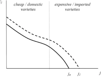
— and imported — varieties increases. Figure 3 illustrates the eect of an income raise.

plotting consumed quantities (vertical axis) against the indexm 5M of varieties (horizontal axis). Varieties are ordered according to ascending prices so that consumption is positive form ? mr only (bold line). An increase in total expenditure at constant prices (a shift to the dashed line) increases consumption levels for m ? m_r and induces an increase formm_r to m₁. When expensive varieties are identied with imported varieties, this implies that the bundle of imported varieties grows and, at the same time, the expenditure share on imports increases.

Finally, notice that the generic demand curve (4) implies that either two varietiesf_lm and flo consumed in positive quantities the identity

1 +flm

1 +f_lo = t_lo

t_lm (5)

holds.

Supply. In each country the nontradable good G is produced competitively with a constant returns to scale technology

G=O_G (6)

The tradable varieties are produced according to the increasing returns to scale technology

O_m =+_m{_m (7)

9The transformation˜f=f@&(& A0) impliesln(˜f+ 1) = ln(1@&) + ln(f+&)and shows that, as long as consumption units are free, the coice of adding unity instead of a positive constant does not mean a loss of generality.

Figure 3: Demand under Bounded Marginal Utility

whereO_m is labor and{_m is output ofrmm. The parameterrepresents an entry cost to production measured in labor units; _m is the marginal unit labor requirement. There is an unlimited pool of potential entrants into the market and each activerm produces one variety. Firms engage in monopolistic competition, and free entry into production ensures that operating prots cover the setup cost.

Pricing. In the competitive nontradable sector prices trivially equal wages. In the tradable sector, rms price-discriminate across dierent countries so that a rm m sets the price s_lm for market l in order to maximize its operating prots _lm in that specic market. When rm m is located in country n and gross iceberg-type trade costs between country n and country l are nl 1, the consumer price in country l of variety m is the t_lm =_nls_lm. In the marketlrm m makes the prot of _lm=O_lnlf_lm(s_lmz_nn), where Ol is the number of individuals in the marketlandz_n is the wage in countryn(i.e. z_nn is the marginal cost of production). With local demand (4), rmm’s prots are thus

_lm =O_lnl(1@(_lnls_lm)1) (s_lmz_nn) (8) Generic prot maximization implies

s_lm=p

z_nn@(_lnl)

for each market lseparately. With the expression (4) this price can be written as

slm = (flm+ 1)zn_n (9) Notice that markup over marginal cost equalsf_lm+ 1, corresponding to the demand elas-

ticity from (4), which equals

%lm= (flm+ 1)@flm= (10)

The demand structure assumed in (2) thus implies that the own-price elasticity of varieties depends on quantities consumed^10>11.

Free Entry. Firms within each country face the same production costs and charge the identical prices in a given market so that the index of the representativerm of a country can be indexed with the country indexn itself. Combining (8) and (9) the prots arm in countrynmakes by selling to countrylare

_ln=O_lnlz_nnf²_ln (11) Under free entry to production, total operating prots, i.e. the sum of a rm’s prots in each market, are equal to setup costs:

X

l

O_lnlnf²_ln = (12)

for all countriesn.

Labor Market Clearing. Consumers spend constant fraction1 on the nontradable good G and, consequently, the same fraction 1 of workers is employed in the non- tradable sector. The resource constraint in the remaining, tradable, sector requires then

q_nh³X

lO_lnlf_ln´

_n+i

=O_n=

Combinign this equation with (12) leads to qn_nhX

lOlnl(fln+ 1)fln

i

=On (13)

for all countriesn. (Notice that formally, summation in (13) runs over all trade partners n, including those with zero exports to countryl(f_ln = 0).)

3.1 Closed Economy

Whenever international transport costs are prohibitive the trans-border trade runs dry.

This case can be analyzed by looking at one representative closed economy, within which

1 0The present paper’s motivation partly rests on the "elasticity-puzzle", i.e. on the discrepancy between measured import elasticities and the observed rise in trade volumes. Thus, a calibration of the model will be necessary to asses the implied import elasticities at observed trade shares.

1 1In line with the estimates in Haveman and Hummels (2004), preferences specied in (2) predict higher markups at higher per capita consumption levels.

transport costs are assumed to be negligible (ll = 1). Dropping country indices, the representative rm in an autarkic economy sets its price according to (9):

s= (f+ 1)z> (14)

its operating prot (11) is

=zOf² (15)

and prots (11) together with the free entry condition (12) determine the quantities con- sumed per individual and per variety:

f= r

O (16)

Equation (16) shows that, quite intuitively, an increase in setup over marginal costs (@) increases per capita consumption of the average variety. At higher values of @, vari- eties are relatively costly to invent, so that less dierent varieties exist and per capita consumption of each of them is high. Conversely, if population size O increases, demand for varieties is high, which increases the number of active rms and reduces per capita consumption of each single variety.

The equilibrium number of activerms, q, isnally determined by labor market clearing (13) and goods market clearing ({=Of):

q= O +s

O (17)

Notice that the number of activerms is determined by technology parameters, the mar- ket sizeand population. The dierence between the two latter parameters is noteworthy.

Market size, dened as total expenditure on varieties (O), enters the number of rms linearly, so that a one percent increase in market size induces a one percent rise in the number of active rms. (This rst eect is the only one under CES preferences.) Pop- ulation size, however, has an additional eect on the number of rms, which it tends to reduce when the market size is held xed.

For an intuition of this second eect, compare two economies, the rst with twice the labor force but half the parameter of the second. Expenditure on varieties f_m is iden- tical in both economies, yet per capita expenditure of the former economy is half of the latter (₁ = ₂@2 and O1 = 2O2). Now, if the number of rms happened to be equal, consumption per capita and per variety in the rst economy would be lower than in the second. Consequently, rm markups would be lower in therst economy as demand elas- ticity decreases with per capita consumption by (10). This, in turn, implies that operating prots would be strictly lower in therst economy, thus violating the free entry condition.

Instead, in the rst economy with higher demand elasticity, and lower markups require

that the total number ofrms be lower. This mechanism explains the negative impact of Oon qin (17) onceOis controlled for.

In sum, the overall eect of an increase in population O on the number of rms is still positive, but, due to the demand eects discussed above, an increase in population size induces a less than proportional increase in the number of rms and thus increases per capita consumption of the average variety.

Before closing this section, it is instructive to consider the necessary condition for autarky to prevail. A given pair of countries does not engage in cross-border trade if at a virtual level of relative wagez^W@z and autarky consumption level (9) consumers in at least one country do not demand foreign varieties. When variables of one country are marked with an asterisk, these conditions are,

f+ 1

1 z^WW

(f+ 1)z or f^W+ 1

1 z

(f^W+ 1)z^WW ; z^W z A0=

where f = p

@(O) and f^W = p

@(^WO^W) according to (16). This condition can be summarized by

³p@(O) + 1´ ³p

@(^WO^W) + 1´

(18) Obviously, when trade costs 1 drop to levels close enough to unity, condition (18) is violated and the two countries engage in international trade. Similarly, when marginal productivity (1@^(W)) in at least one country grows large enough, consumption per capita and per variety (16) in this country rises up to a point where local consumers are willing purchase the more costly foreign varieties. Thus, either reductions in trade costs or rising marginal productivity can generate trade. To analyze either case, consider a two-country economy next.

3.2 The Two-Country Model

Consider a pair of countries and assume that trade costs are low enough or marginal productivities are high enough to generate positive cross-border trade. To simplify the notation the variables of the second of the countries will be marked by an asterisk. Indi- viduals in one country can purchase varieties produced in the other. Yet, for every unit of a variety to arrive at its destination, A1units of it have to leave the producer’s country.

As rms price discriminate between countries their prices are summarized by the pair (s_g> s_i) forrms located in country 1 and (s^W_g> s^W_i) forrms located in country 2. Denote the quantities consumed in the respective country by(f_g> f_i) and (f^W_g> f^W_i). The necessary and su!cient condition for bilateral trade ows to be zero (18) has been derived in the previous subsection. Consequently, under positive trade ows (f_i> f^W_i A0) the inequality

(18) must be violated. If this is the case (16), implies fg+ 1

f_i + 1 s

z^WW

z and f^W_g+ 1 f^W_i+ 1

s z

z^WW (19)

The rst (second) condition holds with equality whenever f_g A 0 (f^W_g A 0). Notice also that together both inequalities imply

f_g+ 1 fi + 1

f^W_g+ 1

f^W_i + 1 (20)

so that, by 1 either f_g or f^W_g is strictly positive. Now, according to (9) the rms’

optimal price in the respective markets are

sg= (fg+ 1)z s^W_g= (f^W_g+ 1)z^WW

s_i = (f^W_i + 1)z s^W_i = (f_i + 1)z^WW (21) and the corresponding prots (11) are

_g=Ozf²_g ^W_g=O^Wz^WW(f^W_g)²

i =O^W z(f^W_i)^{2 W}_i =O z^WWf²_i (22) Free entry conditions in both countries imply

f_g= s

@O^W(f^W_i)²

O and f^W_g= s

@^WO f²_i

O^W (23)

With the prices (21) the trade balance (qO^W s_if^W_i =q^WO s^W_if_i) is

qO^W(f^W_i + 1)zf^W_i =q^WO(f_i+ 1)z^WWf_i (24) The two countries’ resource constraints from (13) are

q£¡

Of_g+O^W f^W_i¢ +¤

=O and q^W[(O^Wf^W_g+O f_i)^W+] =O^W (25) and can be used to eliminate q and q^W in the trade balance. This leads to the following expression for relative wages

z^W

z = f^W_i+ 1

Of_g@f^W_i+O^W +@(f^W_i)

f_i + 1

O^Wf^W_g@f_i+O +@(^Wf_i)

¸₃1

(26) Substitutingf_gf^W_gfrom (23) makes the expression on the right of (26) (the RHS) a function f^W_i and f_i only, which is, moreover, increasing inf^W_i and decreasing inf_i.

Since optimality condition (20) showed that either f_g or f^W_g is strictly positive, the two

casesf_g A0 and f^W_g A 0 are to be distinguished by combining, respectively, the binding conditions in (19) with the trade balance (26). Making use of (23) leads to¹²

O^W

q@(^Wf²_i)3O

O^W +O

¸

^W+@f_i

O

q@((f^W_i))²3O^W

O +O^W

¸

+@f^W_i

=

;A AA AA AA AA

? AA AA AA AA A=

1

μq@3O^W(f^W_i)²

O + 1

¶2

(fi + 1)

³ f^W_i + 1

´ li fgA0

³

f^W_i + 1´

(f_i+ 1) μq@^W3O f²_i

O^W + 1

¶2 li f^W_gA0

(27)

Consider now therst casef_gA0. Iff^W_g= 0, then (23) implies thatf_i is constant so that the RHS of (27) is decreasing in f^W_i while the LHS is increasing inf^W_i. If, instead,f^W_gA0 then (20) holds with equality and (23) implies

r³

@^WO f²_i´

@O^W+ 1

fi + 1 = f^W_i + 1 r³

@O^W(f^W_i)²´

@O+ 1

This equation establishes a negative relation between fi and f^W_i, which implies that the RHS of (27) is decreasing inf^W_i while the LHS is increasing inf^W_i.

In the second case, wheref^W_gA0 holds, considerrst the case f_g= 0, implying with (23) thatf^W_i is constant. Iff_gA0, instead, the logic above shows that the the RHS of (27) is decreasing in f^W_i while the LHS is increasing in f^W_i. Thus, the two-country equilibrium — determined by (19), (23), (25) and (27) — is unique.

Finally, the trade share of therst country ish=q^W s^W_ifi@ h

qsgfg+q^W s^W_ifi

i

. Identities (21) and (24), (26) can be used to eliminate prices, wages, and the number of rms to express the trade share in terms of the equilibrium consumption levels:

h= O^W(f^W_i + 1)f^W_i O(fg+ 1)fg+ O^W(f^W_i+ 1)f^W_i for therst country’s trade share.

3.3 The Multicountry Model

To analyze the general multi-country model, we need to describe the set of varieties an individual in a given countrylconsumes. Sincerms within a country are identical, this set ofrms is equivalently described by set of countryl’s source countries.

1 2In the casefg> f^W_gA0(20) holds with equality and both expressions on the right hand side coincide.

Dening rst the origin country of the cheapest varieties in country las lr =argmin

nML {nlzn_n} the set of countries country limports from is

Pl= n

n5L|fllr+ 1A q

nlzn_n@(lrlzlr_lr) o

(28) where demand (4) and prices (9) have been used. By denition this set of countries that export to country ldoes not exclude country litself. Now, for all n5Pl

(f_llr+ 1)²_lrlz_lrlr= (f_ln+ 1)²_nlz_nn (29) holds. Notice also that the set P_l, comprising country l’s source countries, does not necessarily coincide with the set of countries country l exports to. This latter set of export destinations is

Hl =n

n5L|f_nnr+ 1A q

_lnzl_l@(_nrnz_nrnr)o

(30) The denitions of P_l and H_l rely on equilibrium wages z_n and are, at the same time, outcome of the equilibrium. Combining labor market clearing (13)

q_ll

"

X

n

O_nln(f_nl+ 1)f_nl

#

=O_l (31)

with the trade balance

q_lX

n

O_ns_nllnf_nl =O_lX

n

q_nnls_lnf_ln

and prices (9) leads to

zl =X

n

zn

Onnl(fln+ 1)fln

P

pOp_np(f_pn+ 1)f_pn (32) The multi-country equilibrium consists of a set of consumed quantities {f_ln}l>nML, wages {zl}^lML, number ofrms {ql}^lMLand sets of supplied and supplying countries{Hl}^lML and {P_l}lML. These L(L + 2) variables are jointly determined by equations (12), (28), (29), (31) and (32).

The system (28) - (32) can be solved numerically. It exhibits, however, a complex in- terrelation between the sets of trade partners (Pl and Hl) and wages (zl), which stems from the corner solutions in individual optimization (f_ln = 0 for n 65 P_l). Instead of addressing these di!culties analytically, the paper proceeds by strongly simplifying the

model to symmetry.

3.3.1 Symmetry

Assume that all countries are identical in terms of labor force and technologies. Pairs of countries may dier regarding the respective transportation cost they face when engaging in bilateral trade. Yet, to reap the virtues of the symmetry-assumption, countries are supposed to be symmetric in terms of potential trade partners. In particular, the vector of gross iceberg trade cost _l = (_l1>l2> = = = > _lL) is, up to reordering, identical across countries l.¹³ As all parameters that govern demand and supply are — up to permutation

— identical across countries, producer prices and wages equalize throughout countries and can be normalized: z_l =z= 1.

The bounded marginal utility from varieties implies, just like in the two-country model, that there is a threshold on the transportation cost ¯ above which there is no bilateral trade. The dening condition for this threshold is determined by demand (4), prices (9) and autarky consumption (16)

f_ll=p

@(O) =s

¯

1 (33)

(Compare also (18).) Consider now, say, country 1 as the representative country and denote byP the set of countries it purchases varieties from. Under prices (9) the optimal consumer choice requires

f11+ 1 =s

1n(f1n+ 1) n5P (34) The prots armm located in country 1 makes by selling to market n5P are (11) and the free entry condition (12) is

₁ = X

nMP

_1n= X

nMP

O(f₁₁(s_1n1))²= (35)

Writing the shorthand W_P>1 = X

nMP

(s_1n1) and W_P>2 = X

nMP

(s_1n1)²

condition (35) leads to an expression for per capita consumption of the domestic varieties:

f₁₁= W_P>1

|P| + s

O|P|+

μW_P>1

|P|

¶2

W_P>2

|P| (36)

1 3For alll> nML there is a permutation:L<Lso that(l) =n

Here and in the following, |P| stands for the number of country 1’s trade partners (el- ements of P). Note that P is an endogenous variable that eventually depends on the schedule of bilateral trade costs. Formally, (36) and (37) exhibit a circular denition, as P is dened as

P ={n5L|s

1n? f11+ 1} (37) while f₁₁ depends onP itself. One can show, however, the following

Proposition 1 The set P is non-empty and uniquely dened by (36) and(37).

Proof. Assume wlog that the elements of the vector₁are ordered according to ascending size. Then note that 1o 1n implies n 5 P , o 5 P. Consequently, by (37), any solution to (37) must be of the form {1>2> ===> q} for one q 5 L. Now dene f_q by (36) under P = {1>2> ===> q} and observe that f_q is decreasing in q, so that the sequence dened by pq = max©

n5L|s1n ? fq+ 1ª

is decreasing in q. By monotonicity and since {1} 5 P, there is a unique q^W satisfying p_qW q^W and p_qW+1 ? q^W + 1. By construction the set {1>2> ===> q^W}solves (37).

With the equilibrium per capita quantities of domestic varieties well dened, equations (34), (35), and the free entry condition (q£

+O¡P

nMP1nf1n

¢¤=O) determine the number of active rms

q= O

+O

"

(WP>1+|P|) r

O|P|+

³_W

P>1

|P|

´2

^W_|^P>2_P| +^(WP>1_|P|⁾² WP>2

# (38)

Consumers’ optimality condition (34) and (36) imply that the trade share of country 1 is

h=

1 qs11f11

qs₁₁P

nMPs_1nf_1n

¸

= 5 71 1

P 3

C1 + WP>1

q|P|

O + (WP>1)²|P|WP>2

4 D 6 8 (39) The equations (36) — (39) pin down the representative country’s number of trade partners and its trade share, the two key trade parameters which the present model aims to explain.

The set of a country’s trade partners P depends on the model’s parameters and may be any subset of the full set of countries L satisfying {1} P. Just as in the two- country world, trade costs can, if they are too high, impede bilateral trade. As discussed in connection with generic demand (4), the inclination to pay for more expensive foreign varieties increases with rising per capita consumption of the domestic varieties. Since per capita consumption of each domestic variety decreases with population sizeO(more local varieties exist due to market size eects) while it decreases in the ratio @, one may conjecture that these parameters drive the contraction or expansion of the set of trade partners.

Similarly, the trade share (39) can be expected to fall inOand rise in@— not only since per capita consumption of foreign varieties increase relatively more than domestic varieties (compare (34)), but also because the set of trade partners expands. The dimension of trade partners - or source countries - constitutes an extra margin along which trade volumes expand and amplies therst eect.

The above considerations regarding the number of trade partners and the trade share prove right and the impact of population size and technology on these variables is summarized in the following

Proposition 2 Trade share hand number of trade partners |P|increase in @(O).

Proof. Note rst that for any change in the set P condition (34) must be satised for the newcomer (dropout). Thus, the trade share as h=³

1_|P|f11^f11_3WP>1´

is continuous at any change in |P|. By this observation and by (36) it is su!cient to prove that the equilibrium f₁₁ is increasing in @(O). Using (36), this is trivially the case whenever

|P| is constant. Consider now change — wlog an increase — in |P|. Dene p as the index of the lowest bilateral iceberg trade cost outside the set of trade partners, i.e.

p =argmin_nML\P{_1n}. Whenever |P| increases condition s_1p = f₁₁+ 1 must hold and equation (35) is satised for both of the two setsP andP^{p}, implying thatf₁₁ is continuous. This proves thatf11 is increasing in@(O).

Proposition 2 shows that the rise in trade share and the expansion of the set of trade partners are jointly driven by growth of marginal productivity. If the eect of this joint determinant is strong, it can induce a strong positive correlation between the rises in trade volumes and the number of source countries as exhibited by the data (see Figures 1 to 2).

Moreover, it implies the common dynamics between per capita income and trade volumes (see,e.g., Hufbauer (1970) and Ventura (2006)).

At this point, it is worth to remember that the standard models fail to address these patterns of the trade data, so that the results presented in Proposition 2 constitute an improvement in reconciling the theory with the data. The sole departure from the standard setup was to assume that consumers derive only bounded marginal utility from varieties at zero consumption levels. Finally, to check that these results are qualitatively important it is worth evaluating how the model performs quantitatively.

3.3.2 Calibration Exercise

To assess how the model performs quantitatively, a symmetric version is calibrated to US trade data; the number of countries is 20. This choice requires a word of justication. On the one hand, models that re ect relative economic sizes do better in predicting trade

volumes since the share of world output is a key determinant of a country’s trade volume (see , e.g., Anderson (1979)). On the other side, the number of source countries is a key variable of the present paper’s model, which requires the number of potential trade partners to be relatively large. With a su!ciently large set of countries, however, the calibration of the asymmetric multi-country model cumbersome and intransparent. For this reason, I resume to the symmetric model.

Imposing symmetry is of course a heavy simplication. Yet, in defense of this assumption one may remember that relative per capita income between countries is very stable in the long run (see Acemoglu and Ventura (2002)) and that, as long as PPP holds, real exchange rates do not change dramatically (see, e.g., Froot and Rogo(1996) or Wu (1996)). Since, nally, the ultimate channel through which country size aects trade volumes operates through terms of trade movements, these observations suggest that the error of imposing symmetry be limited. Thus, as a compromise that accounts for the number of source countries as well as for trade volumes, the world is assumed to consist of 20 countries — a choice that re ects the US share of world population, ranging around 5% throughout the time interval considered.

Turing to the calibration itself, the parameter is normalized to one and the units for population O are set to millions. Both choices in ict no loss of generality since the ratio

@(O) is the only relevant variable for the calibration of the number of trade partners

|P|and trade sharesh (see Proposition 2). Hence, the model is left with the parameters , and trade costs _1n, which are to be calibrated to US data. Key time series are US non-oil import share and imported varieties, both derived from data as described in Feenstra et al (2002).

The calibration follows Yi (2003) to match the US trade share in the initial period (1972) with the choice of parameter . Similarly, the trade share of the nal period (2000) is matched with the adequate choice of the initial productivity parameter₁₉₇₂.¹⁴ This leads to = 0=15 and ₁₉₇₂ = 14=39. Next, population size and per capita income are from Penn World Tables 6.2. The latter series is used to proxy growth in marginal productivity (1@).

Bilateral trade costs are assumed to be the sum of trade-weighted taris (taken from Feenstra et al (2002)) and the cif/fob measure (from the IMF International Financial Statistics). Anderson and van Wincoop (2004) estimate an ad valorem border cost of 40%, which is added. Total trade costs are assumed to be additive between taris w and transportation cost and are assumed to take the form p = 1=4 +w+(p@(P1)). The functional form of the last term is chosen to t the US bilateral trade cost data from 1989 to 2000 for 20 trade partners with the largest export volume to the US (data

1 4The joint choice ofanddetermines consumption units; compare also footnote 6.

0246810Trade Cost (Percent)

0 5 10 15 20

Rank

20 Trade Partners with Largest Trade Volume

Fit of Trade Costs

Figure 4: Trade cost for US trade partners with largest exports to US.

described in Feenstra et al (2002)).¹⁵. Figure 4 shows that this functional form provides a goodt for the trade costs data. The parameter is chosen so as to maximize thet and is set to = 1=9 (the corresponding adjusted R-square including time dummies is0=897) For each period, the value is chosen so that the cif/fob measure implied by the model coincides with the data. Table 1 summarizes the calibration of the key parameters; time series of population, per capita income, taris and trade costs are listed in the Appendix.

Table 1: Parameter values; calibrated to 20-country model.

As stated above, the model is calibrated to match the increase in trade shares so that its success in matching the data will be assessed along two main dimensions. The rst dimension concerns the implied import elasticity. Yi (2003) puts forward that the increases in world trade volumes imply an excessive import elasticity in conventional models. Thus, import elasticity with respect to taris is a parameter of key interest in the calibration.

It is here dened by

E=(1 +w)g gwln(T)

where T stands for the total imported quantity. With prices (9), the optimal consumer

1 5A list of countries is in the Appendix. Data on bilateral trade costs as in Feenstra et al (2002) are available only for the period 1989-2000, wherefore this data source of trade costs is not used directly.

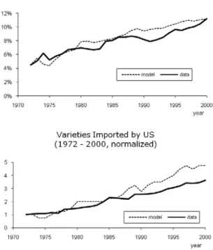
Figure 5: Data vs Model: Import Shares (top panel) and Number of Varieties (bottom panel).

choice (34), and the number of rms (38) this is T=q X

P\{1}

f_1n=

à (f₁₁+ 1)P

P\{1} I11n (P1) +O[f₁₁(W_P>1+P)W_P>2W_P>1]

!

With this denition, the implied import elasticity has a time-average of3=7with a peak of 8=8at the start of the period and a minimum of 1=75at the end of it. While the variation is arguably high, this time-average is close to the interval [2>3], which Yi (2003) puts forward as a realistic range. At the same time, the top panel of Figure 5 shows that the model’s track of trade shares is reasonably close.

The second dimension along which the model should perform is the number of source countries. The bottom panel of Figure 5 graphs the number of imported varieties, dened as goods dierentiated by country of origin (values are normalized to one at the initial period)¹⁶. The model’s prediction exceed the data by a factor of1=4. This prediction not terribly precise but neither is it completely othe mark. For a stylized and dramatically simplied model its overall performance is reasonably satisfying.

1 6As in Broda and Weinstein (2004), varieties are dened as good dierentiated by country of origin.

Data are as described in Feenstra et al (2002). Good categories are dierent from those underlying Figures 1 and 2. In particular, they rely on TSUSA classication for the years from 1972 to 1988 and HS classication from 1989 to 2000.