The main topic of this thesis is how to solve large exhaustive graph search problems. A search problem is called exhaustive if its solution requires us, in general, to visit all its nodes.
Search Problems
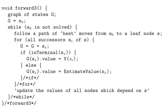
To calculate the value of the starting state, we first solve for all successors and then propagate the values. Another difference is that backward search returns a value for each state, while forward search returns only the value of the starting state.
Games as Search Problems
A game is called convergent if the size of the available state space falls below a game. In the previous section, a search problem was solved as soon as the value of the initial state was known.
State of the Art
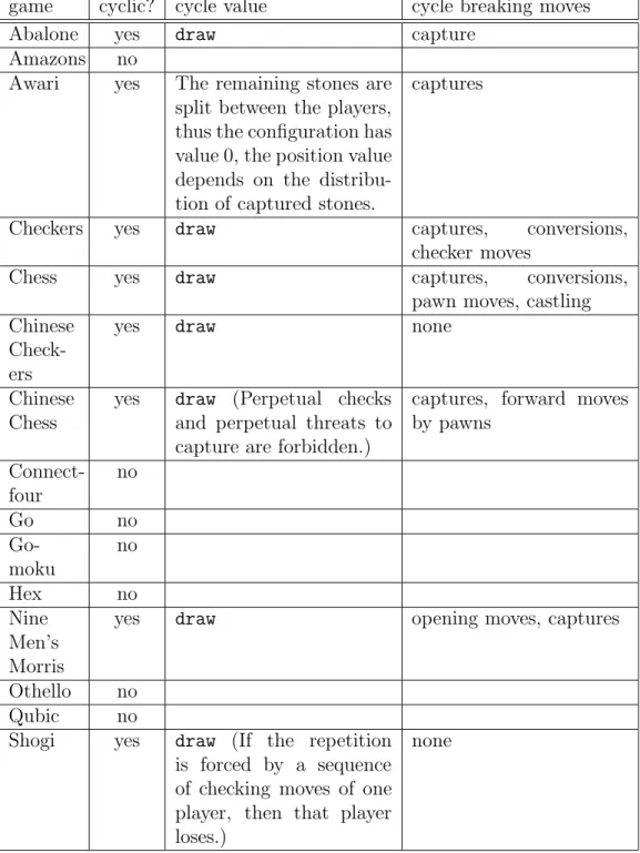
An interesting observation about the above list of solved games is that the year a game was solved and the size of the game seem to be unrelated. In Nine Men's Morris, only the subspace after the opening is cyclical; that part of the game was solved with backward search.
Contributions
Dropout Expansion: When putting together an opening book, we need to decide which positions should be part of the book and which should not. We estimate that Awari's solution would require the completion of at least the 44-brick database, meaning that more than 50% of the state space of approximately 0.9∗1012 positions would need to be fully enumerated.
Thesis Overview
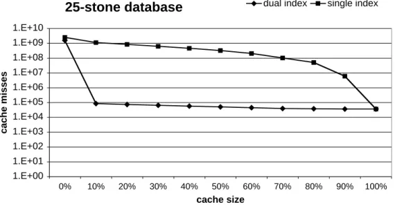
This chapter introduces a new double-indexing algorithm that significantly improves disk I/O performance in backward searches when the state space of a search problem does not fit in main memory. Due to the popularity of the game, most of the research for retrograde analysis has been done on chess.
Retrograde Analysis for Awari
Of course, the assumption that the value of the best move will only increase is weak. If he keeps playing good moves, we won't be out of the book early. However, the candidate set of leaf nodes changes most radically when the value of the start node changes.
We are not interested in the value of the starting node; we are only interested in the best move. Using the new propagation rule, we can prove that the value of the starting position is a tie. This is due to the fact that the vast majority of positions in the book have 40 or more stones on the board.
This ensures the utility of the opening book regardless of how the opponent plays the opening.
Two Bits per Configuration
One Bit in Memory
In the second case, the configuration may contain some non-capturing moves that may later turn out to be winning moves. In the post-processing phase, we examine each configuration again, and merge the corresponding memory and disk values into the configuration value.

Beyond One Bit per Configuration
The Choice of an Algorithm depends on Memory Size
Another drawback is that the method only applies if there is any human opening book knowledge in the first place. If the opening book is stored as a directed graph, with positions as nodes and moves as arcs, then the values can be propagated within the book.
Opening Book Basics
Book Representation
Book Expansion
Goals
Drop-out Diagrams
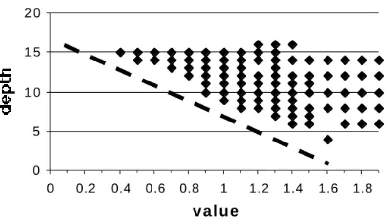
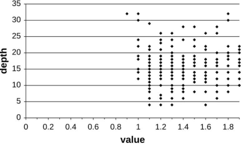
Or to rephrase the question if you were against the book player: Which leaf node would you try to reach. Obviously, if the opponent plays only the best moves, the book player will be able to play at least 32 suits from the book. However, as the plot shows, there is a line in the book that ends at layer 4 with a value of 1.1, which is only 0.2 points worse than the best value.
Expansion strategies
- Best-First Expansion
- Drop-out Expansion
- Further Enhancements
- Other Considerations
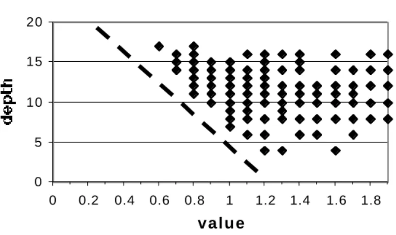
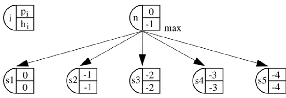
It is initialized to zero in the leaf nodes and depends only on the expansion priority of the best successors. As the depth of the best move increases, so will the priority for extending the suboptimal moves. An additional advantage of the discharge expansion is that the parameter ω can be used to control the shape of the opening book.
Conclusions
Partially Ordered Sets
Since the draw value and the heuristic values are incomparable, the set of game position values forms a partially ordered set [47, Chapter 3]. The Hasse diagram of a partially ordered set P is the graph whose vertices are the elements of P, whose edges are the coverage relations, such that if x < y then y is drawn.
Workaround for Search Engines
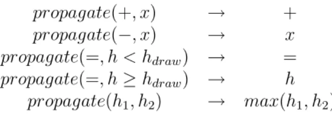
Whenever we compare a draw with a heuristic value h, we propagate draw if h < hdraw, and we propagate h if h ≥hdraw. This means that the higher the value of hdraw, the higher our preference for a draw. This solution is cheap and useful for search engines, but not useful for creating opening books because we don't know the value of hdraw at the time of build.
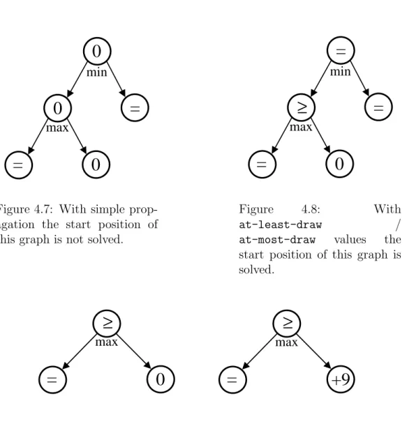
At-least-draw and At-most-draw
At-least-draw, At-most-draw and Opening Book Con-
This is exactly what drop-out expansion does: ≤|a is treated as 0, and the expansion priority of the two features depends on the depths of the subtrees. However, the value of the start node does not depend on a, so expanding the left node is unlikely to affect the value of the start node. Solve the game There are several ways how the starting node in figure 4.12 can be solved in whole or in part.
Cycles
Cycle-draw
As indicated by the use of + and − in the cycle drawing notation, the first attribute is always strictly positive and the second attribute is always strictly negative. Then the value of the move leaving the cycle is assumed to be better and the corresponding heuristic value is passed. We conclude that the cyclic drawing values are generalizations of the previously introduced values of minimum drawing, maximum drawing, and drawing.
Cycle-draw and Book Expansion
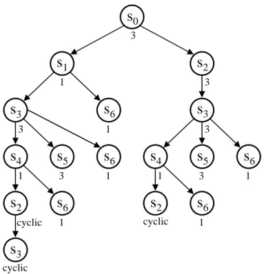
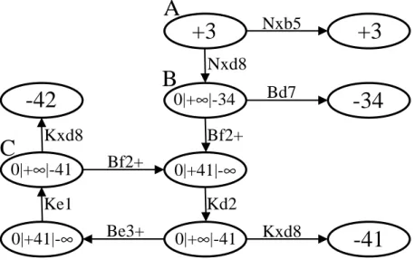
We use 0|+| −h for the case where the opponent only has lost moves to leave the cycle, we use 0|+h|− for the case where the current player only has lost moves to leave the cycle, and we use 0|+|− for the case where both players lose if they play the cycle of the leaving move. We have solved this problem by using a drop-expansion strategy, where the priority of expanding a leaf node depends not only on its value but also on its depth, see Section 3.4.2. For example, if we are in position A, we cannot decide locally which move leads to the best moves to exit the cycle (leaf nodes with values +1 and +2).
Cycle-draw and Tournament Play
The motivation for implementing OPLIB was twofold: First, due to the lack of human expertise in Awari, we needed a tool to automatically create the opening book. Second, because of the observation that the previous game solution always involved some extensive forward search. However, it also requires certain maintenance costs because we have to keep track of the recursive work breakdown and the reconstruction of the results.
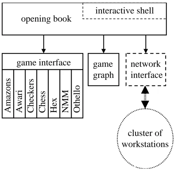
Implementation
Main Memory versus External Memory
Most ledger operations only require access to a position or a path of positions. Keeping the book on disk makes system startup time independent of the size of the book. The drawback of this approach is that the operating system knows nothing about the semantics of the data.
Transposition Detection and Cycle Detection
For example, it accesses files block-wise, while in the case of an open book it is preferable to use cache by position, because the book is accessed in staggered positions. Looking back we can say that the decision to save the book on disk was justified. This cycle detection is called manually whenever the book appears to be suffering from too many undetected cycles.
Distributed Expansion
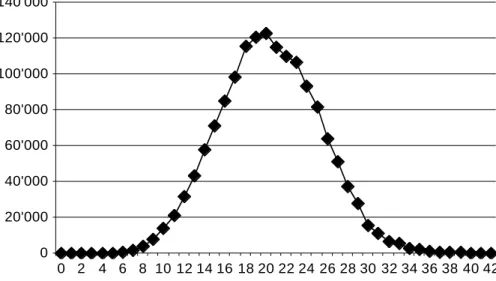
If all values of the cycle-exiting moves are lost, the values of the nodes in the cycle will be these nodes. An upper bound on the size of the state space of Amazons on an nxn board is2. The branching factor is very high at the beginning of the game, but drops significantly during the first few moves.

Awari
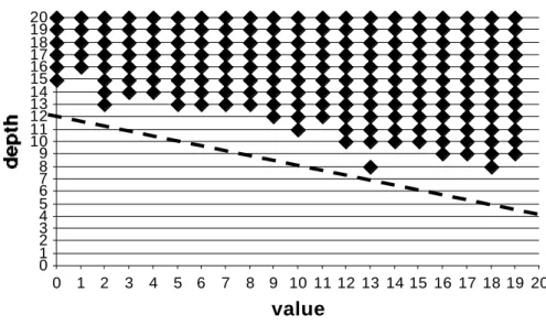
Endgame databases of up to 40 stones were used, but only on the first 8 layers of the search, because accessing the databases at deeper positions would increase the search time without appreciable benefit. The dashed line is the angle of the expansion boundary as defined by our choice of the parameter ω. Construction of the Awari Opening Book started when the 30-stone database was available and continued until the 40-stone database was available.
Checkers
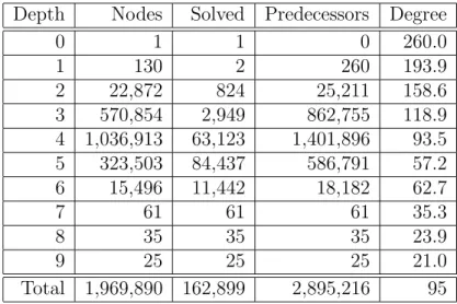
Of course, the engine together with the 6-stone database cannot solve the positions in the early opening. The 'Ancestors' column shows that, on average, each position in the book has about 1.2 ancestors who are also in the book.
Chess
The 'Solved' column shows the number of nodes that were solved, their number is insignificant compared to the total number of nodes in the book. The Predecessors column shows that each position in the book has, on average, about 2 predecessors that are also in the book. To compare the size of our book and human opening knowledge, we need to use the additional observation that the branching factor of principal variations in the human literature is close to one.
Nine Men’s Morris
In that case, we suspect that the game will be solved “for all practical purposes” before any proven value will be known. Most leaf nodes are located at depth 9, because the search engine is configured to resolve these positions with 9-layer searches in the endgame databases. As a side effect, we confirmed Ralph Gasser's previous result that the game is a draw[15].
Othello
When applied to retrograde analysis in the game Awari, the new algorithm significantly reduced the number of disk accesses with good performance even when only 10% of the state space fits into main memory. If the opponent plays bad moves, we may fall out of the book earlier, but we will leave the opening book in a superior position. If the last stone in a move falls into an opponent's pit containing two or three stones (including those just dropped), these stones are.