We introduce a notion of the limited universe and prove lower bounds in that setting as well. However, this does not help the fact that the size of the array can be significantly larger than n.
Applications
We know that in the case of polynomial size arrays, the answer is negative. We know that in the case of linear arrays the answer is also negative, but what about larger arrays.
Definitions
Label Space vs. Array Notation
Organization of the Thesis
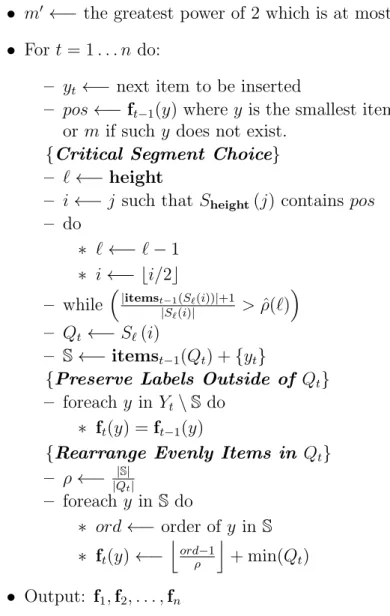
At the very beginning of the round, the algorithm is provided with the next item y to insert. It then finds the appropriate part of the array (segment) that contains this point and finally rearranges the items in this segment (including y) as evenly as possible.
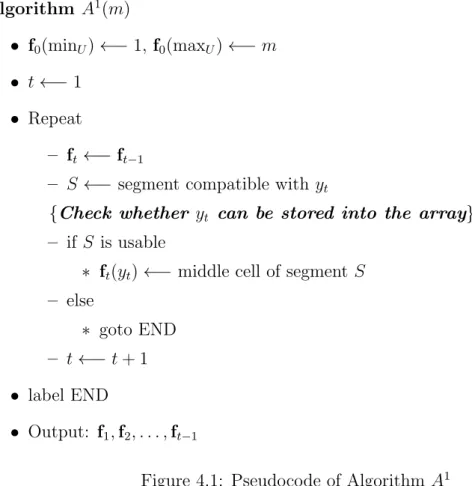
Algorithm Outline
In section 3.3 we state the main theorem of the chapter, which will be an immediate consequence of Lemmas 3.6.1 and 3.8.1. Then we find the smallest segment of the array which contains this point and whose density of elements in it is less than a certain threshold defined for segments of different sizes.
Main Result
Definitions
Segment Hierarchy
Note that the segment hierarchy can be thought of as a binary tree in which each segment (except the last level) has two subsegments and each segment has one parent (except the 0th level). Finally, let's emphasize that the segment hierarchy is not explicitly built by the Asmall algorithm and is used only for the explanation of the Asmall algorithm.
Algorithm Construction
It is easy to observe that boundaries of each segment of the segment hierarchy can be computed in constant time if ` and i are given. Now we can find so-called critical segment Qt which is the smallest segment in the segment hierarchy that contains the position where we want to insert and whose density (with respect to t) is smaller than the threshold density of its level.
Proof of Lemma 3.6.1
We say that segment S is rebuilt at step t if S ⊂ Qt (not Qt itself). In the following proof, we first define how we divide the cost of each step among the items from the paying set at step t.
Modification of Algorithm A small for Very Small Arrays
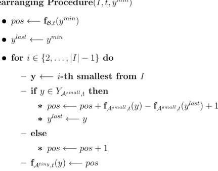
Let YB,n0 indicate the set of items inserted into the array before the algorithm starts. We define the allocation fB,n0 as an allocation obtained by applying the rearrangement procedure (Figure 3.2) with parameters I = YAsmall,n0 and ymin = minU.
Algorithm Outline
In this chapter we present an algorithm for the online labeling problem which achieves the asymptotically optimal time complexity O(n·log logm−log loglogn n) for the label space m ∈ [nlogn,2n] where c is a constant greater than one.
Main Result
Definitions
Algorithm Description and Analysis
There were only two results: a tight lower bound for sets of polynomial size (which of course also holds for smaller sets, but provides a non-tight bound) Dietz et al. In Chapter 6, we present a tight lower bound for deterministic algorithms using arrays of size nc (c > 1) to 2n.
Definitions
Proof Techniques
The hope is that loading many items with value in the middle of the array of items stored in the smallest nested segment will eventually force the algorithm to make expensive rearrangements at many different scales. The advantage of the dual display will be apparent in the case of randomized labeling, where we know what the inserted elements are, but we do not know their particular location in the array.
Lazy Algorithms
The way we choose such subsegment differs between the adversaries, but the basic idea is always the same: we try to detect the density in the array. A dual view is to recursively select subintervals of inserted items that span the shortest possible segment (i.e., the highest density segment).
Introduction
The Main Theorem
Reducing Prefix Bucketing to Online Labeling
At each step t, the adversary determines a certain level pt of the chain as the critical level (which is always at most k =dlog(m+ 1)e). Therefore, the lower bound on the cost of sorting prefix n elements into buckets will represent the lower bound on the cost of the algorithm against our adversary.
An Improved Analysis of Bucketing
Adversary Construction
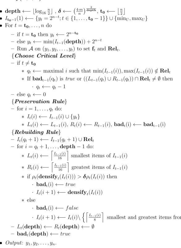
We start by setting limits on the size of the smallest interval in the chain. Next lemma is an immediate corollary of the previous claim and the termination condition of Rebuilding Rule.
Prefix Bucketing
Connecting Bucketing to Online Labeling
This lemma really proves too much, but it nicely illustrates the connection between labeling and bucketing. This follows immediately from the previous lemma and from the fact that It(qt) = {yt} ∪It−1(qt).
Lower Bound for Bucketing
The cost of any prefix buckets of n items in k buckets is at least 8(log 8k−log lognlogn n)−n. Finally, we prove a lower bound on the cost of any strategy for the bucket game, thus giving a lower bound on the cost of the algorithm on the hard input range.
The Main Theorem
The argument relating the cost of A in the hard sequence to the cost of a bucket-bound strategy does not work for the original version of the bucket game, and we can only establish the connection with a new variant of the bucket game called tail-bucket. Finally, the proof of the lower bound for the cost of any bucket hedging strategy is quite different from the previous lower bound for the original version of the bucket.
Mapping a Randomized Algorithm to a Hard Input Sequence
The chain at step t ≥1 is constructed from the chain at the previous step t−1 and the expected behavior of the algorithm at y1,. This construction of the chain is similar (except we don't have two kinds of segments) to that used in Chapter 6 in the deterministic case.
Bucketing Game
We can prove that the minimum cheap cost of tail bucketing is Ω(nlog(n)) if k = O(log(n)). The lower bound evidence for the cheap cost of tail buckets has some interesting twists.
Adversary Construction
A by a deterministic algorithm A in lowercase to indicate the value of the random variable when A=. For each endpoint of Tt(i+ 1), its label remained the same under each of the functions fs,.
Prefix Bucketing and Tail Bucketing
In cheap bucketing, the cost is the number of items in bucket p before the placement:. Inexpensive bucketing, the cost is the number of items in bucketspor higher before the placement:.
Tail Bucketing and the Online Labeling
The following lemma is used to relate the cost of online labeling to the tail sampling. This holds because pt = ¯qt and so ¯j ≥ pt, and therefore Bt is obtained from Bt−1 by adding a single element at position pt and redistributing elements among the first pt buckets so that the difference in the two sums is actually 1.
Lower Bounds on Tail Bucketing
As mentioned, this gives an upper bound of 0 if the number of buckets is at least log(`+ 1). We now show that a small reduction in the number of buckets is enough to give a good lower bound on cost-cheapness.
From cost b−block to cost cheap
We could also define ∆hv(h)+1, but we won't need it.) The sum of the difference series is just hv(h)−h0. For all other relations, we fix an h ∈ H and show that it holds term by term.
Hard Sequence Construction
Ideally, we should build the chain so that the density of successive intervals of the chain does not decrease (which is not necessary in Chapters 6 and 7). We show that in the worst case we can find a large subinterval whose density is significantly higher than the density of the whole interval.
Charging Scheme
This approximates the size of the range buffers divided by the number of items inserted into the level since the last rebuild. This follows from the fact that the number of good levels at each step is a constant fraction of the chain depth.
The Main Theorem
First, we show that the cost of the algorithm at each step can be lower bounded by the number of items in well-interval buffers rebuilt in that step. This is also the reason why we only consider the last half of the items that have been rebuilt since the last time, because for them we can estimate their charge well.
Adversary Construction
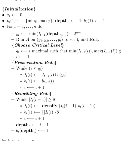
We build the intervals for the chain in step t in order of increasing level (ie, decreasing size). To specify which intervals are preserved, we define a critical level qt for step t, which is at least 0 and at most depth, which is the length of the chain at each step t, t ≥ t0.
Interval Chain Properties
Next two claims show that "badness" and the span of the interval are preserved if the interval is not rebuilt. So from the construction of the adversary and since badt(i) isf asewe can deduce thatρt(L0)≤δ·ρtb(Itb(i)) andρt(R0)≤δ·ρtb(Itb(i)).
Relating Charge to Online Labeling Cost
For t0 =tb this is immediately true as follows from the construction of the adversary. Together with the facts that A is lazy,Ltd−1(i)∩Reltd 6=∅and ytd is inserted "into" Itd−1(i), it follows that such are in Reltd(i).
Estimating the Charge
A lower bound for the small space regime of smooth algorithms is obtained by considering a trivial adversary that inserts elements in descending order. This lower bound obviously depends strongly on the smoothness of the algorithm; a non-smooth algorithm easily copes with a given adversary with a constant amortized time per element.
Proof Techniques
To identify S0 we maximize some quality function of the form ρ(I)|I|κ (where ρ(I) is the density of items stored in I and κ is a small positive parameter). In a given step, after selecting the chain, the opponent is supposed to choose the next item to insert as an item that is between two items currently stored in the last segment of the chain.
The Main Results
How large must r be for the adversary described above to avoid this problem. For this lower bound, we only need the sequence of elements to be polynomial inm.
Reduction of the Theorems to the Main Lemma
We now fill in the (routine) details of the above sketch of the proof of Theorem 9.3.2. This setting of parameters is enough to prove the first part of Theorem 9.3.2 in the case that N = Θ(m) and captures most of the difficulty of the proof.
Some Notation and Preliminaries for the Proof of the Main Lemma 106
The selection of a suitable segment in step t will depend on the configuration (Yt−1,ft−1). In formulating our adversarial strategy for proving Lemma 9.4.1, we will ensure that (in the case of a small gap) the segment chosen by the algorithm satisfies the lemma's hypotheses about the corresponding gap.
Important Properties of the Adversary
This concerns the way in which we will account for the cost of the algorithm, and describing this property requires some additional terminology. The parameter α is closely related to the adversary's input parameter κ (which determines the quality function).
Proof of Lemma 9.4.1
Proof of Lemma 9.7.1
After discussing the previous subsection, we return to (9.15) and try to show that P. What we will do is consider the segment density Tt(i+ 1) with respect to the density function ρs−1 used during step s .