q g m - centre f o r quan t u m g e o m etry o f m o dulis p a c es

In the first part of the thesis, a review of objects and mathematical theories related to the project is presented. In the second part of the thesis, we present new results related to the study of protein structures.

Protein and the folding problem

Protein folding problem and fatgraph model of proteins

One advantage of the fatgraph model is that one can use the tools developed in mathematics independently of what is being modeled. One interesting aspect of this summary is that the class of RNA structure called shapes is in one-to-one correspondence with the cells in a decomposition of Riemann's modulus space of a surface with one boundary component [8].

Content of this thesis

We then conclude the section with a brief discussion of the results of the two algorithms (section 6.5). The number of half-edges incident on a vertex is called the valency of the vertex.

The Penner-Strebel decomposition

We now define a slight generalization of the Teichm¨uller space, called the decorated Teichm¨uller space. The boundary C inside L+ consists of a countable set of "faces" of codimension 1, each of which is a convex hull of a finite number of points in B. The edges ∂C inside L+ have ends in B. Ifz, w∈ Two free ends of the edge, the geodesic line inD, connecting ¯z,w¯∈S∞1 projects onto the geodesic line connecting the corresponding vertices of Fgs.

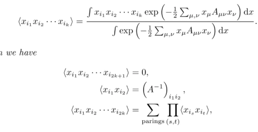
Matrix model

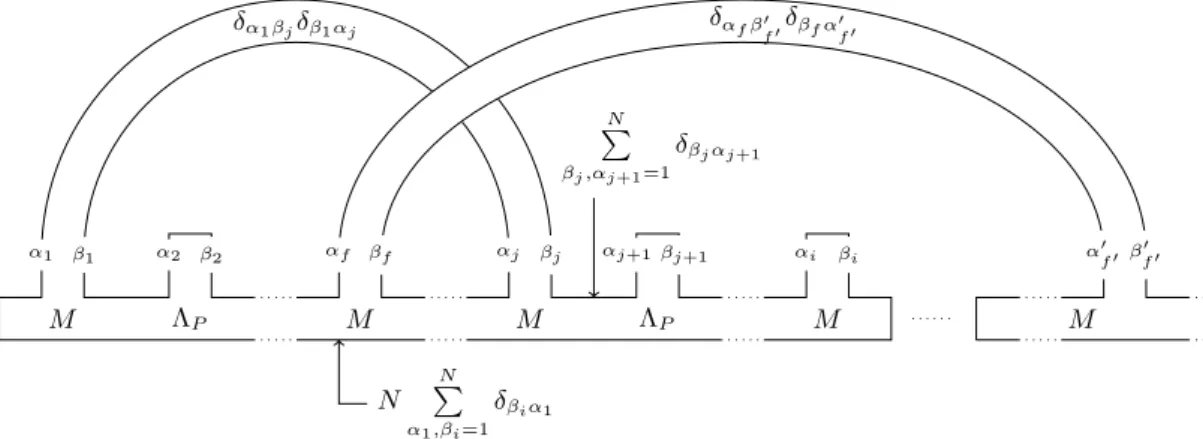
We can generally obtain the number of fat graphs with one-valent vertex in this way. For the power of N, we have a negative contribution of 1/N in the Wick contraction which counts the number of edges.

Topological recursion

Formal setup

Graphically, we can represent the second term in the δikδjl propagator with a twisted band. A symmetric, holomorphic form ω0,2∈H0(U2, KU2(2∆))S2, where KU2 denotes the tensor product of the attracting bundles as defined above, and 2∆.

Topological recursion and matrix models

Moreover, the gender of a shadow is equal to the sum of the genders of its irreducible components; An RNAγ structure is a partial chord diagram S such that the genera of the irreducible components of π(S) is bounded by γ, i.e.

Recursion relation for RNA model

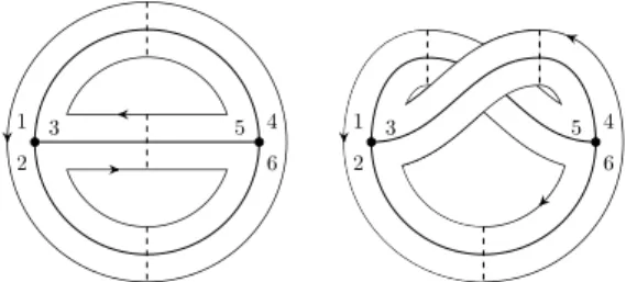
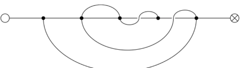
We say that a diagram is of a certain type if it has the specified parameters and spectra; for example, a diagram of type {g, k, l;b,m} has genusg,kchords, lmarked points, with the backbone spectrum band the limit length and the point spectrum m (see Figure 17 for an example). The former is straightforward; given a diagram of type {g, k, l,b,l}, there are kchords to choose from for selection, so this gives l.h.s. We do the latter by first removing a chord from a diagram of type {g, k, l,b,l}(“cut”), and then adding an appropriately marked chord (“join”).

Enumeration of RNA chord diagrams via matrix models

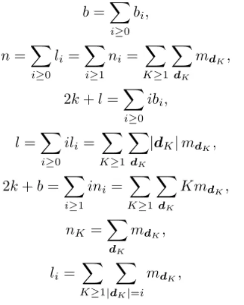
Let us first consider the number of partial chord diagrams filtered by the boundary point spectrum l = (l0, l1, . . .), where li is the number of boundary components within the marked points (a marked point is found in the boundary component that runs above it). The above rules imply that all partial chord diagrams with backbone spectrum b correspond bijectively to all correspondences between M's in the Gaussian mean expansion. The corresponding generating function for connected and disconnected diagrams is given by the exponential;.

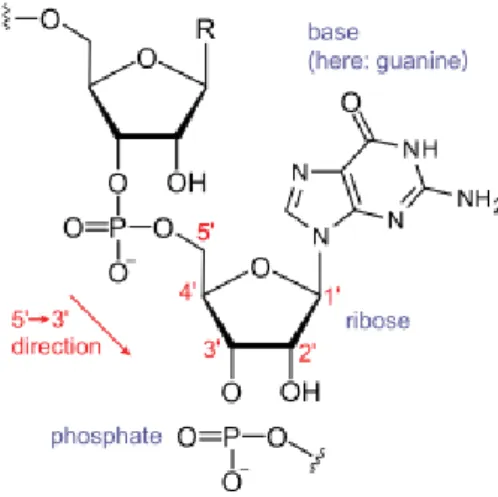
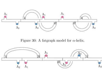
The protein model

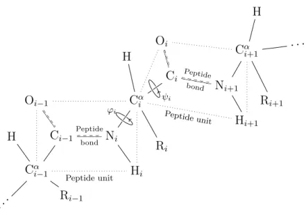
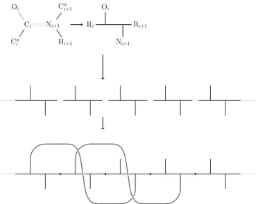
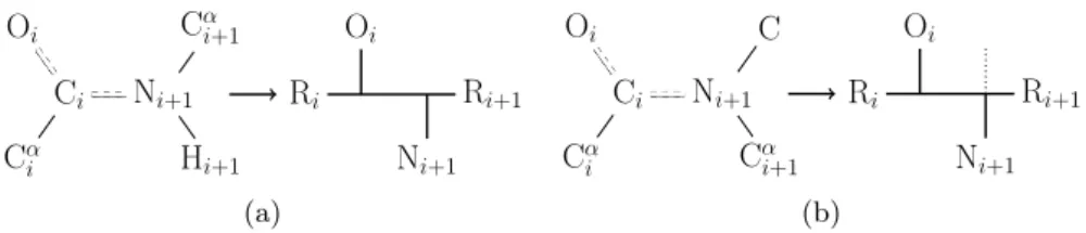
Note the orientation of the backbone from the N- to O-terminus and of the hydrogen bond from the N-donor to the O-acceptor. Let ¯v be the projection of the vector −−−→CαiCi onto the subspace Ru⊥ and setv= ¯v/k¯vk. The choice was made so that we could take advantage of the computational efficiency of expressing fat graphs as a few permutations (section 2.1), and as a purely combinatorial and discrete object, it was expected to be easier to work with.

Recursion relation for the protein model

If we assume that the signatures of the two boundary components after the removal are pK andrL, the original boundary component had the signature. Note in the second case that the chord to be removed must be adjacent to a single boundary component, otherwise the two boundary components adjacent to the removed chord will merge after the removal, which is absurd. If the two components after the removal have signature spK andrL, the single boundary component has the signature before the removal.

The protein matrix model

The heat equation for the partition function ZN(y;α,β,rij) is obtained by the shift invariance of the matrix integral measuredAanddB. By the chain rule applied to the right-hand side of the heat equation (44), we find. We note the first cut-and-join equation (53) expresses the cut/join manipulation of the hydrogen bonds, while the second cut-and-join equation (54) is for loops (or turns) in the backbones.

Protein metastructure

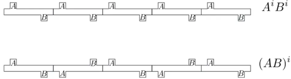
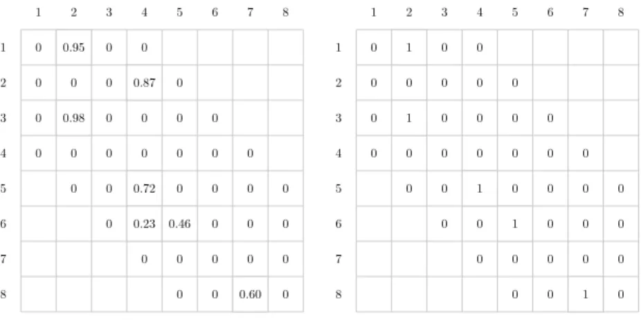
We can make this canonical by requiring the top string to come before the bottom string in the backbone sequence. The 1s in the upper triangular part show parallel pairings, and the 1s in the lower triangular part show anti-parallel pairings. Configuration of the remaining strands in the sheet is determined by the information about parallel/anti-parallel pairings.

Protein metastructure and fatgraph

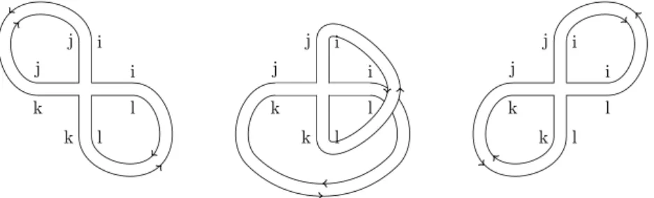
Note that if T is the set of metastructure diagrams, the map ϕ: ˜S → T described above corresponds to “forget”rin (r, P, A)∈S˜. Note that this map ψ from T to the set Σ of fat graphs with two labeled half-edges is not injective (figure 42). Nevertheless, the composition ψ◦ ϕ allows us to calculate topological invariants, such as genus and number of boundary components for protein metastructures.

Recursion relation for extended metastructure

Let , m , and denote the gender, number of threads, and number of thread pairings for a metastructure diagram. We also define the boundary point spectrum n= (n0, n1, n2, . . .), where is the number of boundary components containing odd sides. In the representation in Figure 45, the number of unpaired sides is counted when a boundary component traverses a string over the backbone.

Topological characteristics of protein metastructures

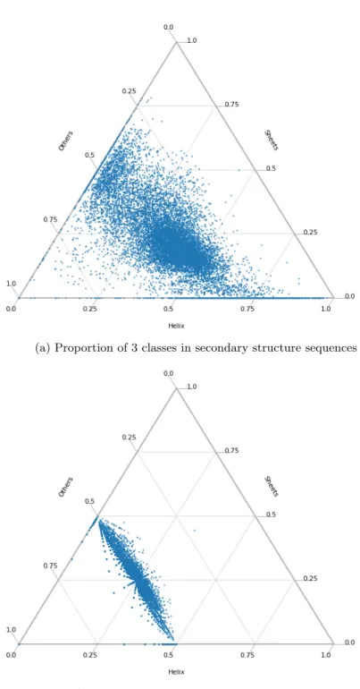
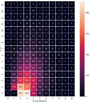
If the sequence has an odd number of letters, the letter "γ" was appended to the end. This implies that metastructures whose associated surfaces have lower genera are preferred over those that result in high genera in nature. For later use, we calculate the distribution of the actual protein data by genus, number of boundary components, and number of β-strands in the largest β-sheet.

Dataset

For each reduced sequence generated as above, a fatgraph structure was assigned as follows. a) Let U be the set of letters in a given sequence, indexed by their positions in the sequence; β1, β2, . We will use the protein metastructures, not the extended metastructures, for the purpose of the current analysis. This choice was made because it was not possible to obtain the extended metastructure information from the reference software we used for the analysis, Betapro [29], as well as for the ease of programming the model.

Applications

• Binary classification of candidate structures by their topol-
• Metastructure prediction by sequence alignment and topol-
• Metastructure prediction by Betapro and topology
• Results

The result is a number of candidate matrices, the number of which depends on the partial pairing matrix calculated in the first part of the method. Let g, n, l denote the gender, the number of boundary components, and the number of strands in the largest sheet. There are large variations in the number of candidates between proteins with the same number of strands.

Discussion

Although the result is skewed by a very uneven distribution of the number of candidate structures per protein, and the acceptance rate response to an increase in quality is not linear, it appears that the topology of protein metastructure captures some information about the original structure. This suggests that a "finer" filter, which can distinguish between structures with the same genus and number of boundary components (and maximum sheet size), might give a better result. We have shown in this project that the topological invariants such as genus and the number of boundary components can describe certain aspects of β-sheet topology of proteins and how they can be used for the prediction of β-sheet topologies.

CASP and GDT

In CASP10, on which this analysis is based, the best performing predictor had an average ∆GDT of 4.6 GDT TS points and could identify a candidate with ∆GDT<2 about 33% of the time [55]. In CASP12, the last round reporting this metric, the best performing predictor had an average. The best performing predictor was able to identify a candidate with ∆GDT<2 40% of the time [56].

Dataset

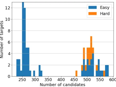
One of the experiments in CASP, conducted since CASP7, is the model quality assessment, where participants are asked to rate the quality of all submitted models [57]. In CASP, participating models are judged based on the difference between the GDT TS score of the candidate identified by the model as the best and the best candidate. The range of the number of candidate structures per protein was from 228 to 584 (entrants may submit more than one candidate structure).

Linear regression based on the protein fatgraph model

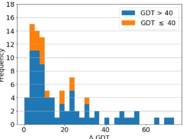
Indeed, there were 47 targets with a candidate count of less than 400, of which 47 had a candidate with a GDT TS higher than 40, while of the 44 targets with a candidate count of more than 400, only 27 had a candidate with GDT higher than 40. This may be the result of fewer submissions for easier targets, as participants are more confident about their prediction, while for more difficult targets, the number of submissions was greater, reflecting growing uncertainty. The average difference in GDTs of the best candidate and our prediction (∆GDT) was 5.52 (figure 56).

GDT-like algorithm based on the protein fatgraph model

Let Dsub(i) be a subgraph of D obtained by taking three vertices {wi, wi+1, wi+2} and the edges connecting them in D. Let Tsub2(i) be a subgraph of T that it is obtained by taking Tsub(i) together with all the edges connected to the nodes in Tsub(i) and the endpoints of those edges (ie "increase" the subgraph by 1 edge + node pair) . If d(i) < r, "grow" the subgraph Dsub(i) by one edge/node pair by selecting all edges connected to vertices in Dsub(i) and the terminal vertices of those edges.

Discussion

It is a subgraph, centered around the hydrogen bond, of the graph consisting of the backbone and all hydrogen bonds in a protein. The central bond determines the signed length of the bond, which is the distance, measured from the donor to the acceptor, between the central. If the distance between the two endpoints of the central bond is greater than 2w, the H-bond pattern is not connected, which can be indicated by.

Rotation prediction by H-bond pattern matching

Method

Thus, for each hydrogen bond in the training data set, we obtain multiple H-bond samples, one for each parameter combination. For each of the remaining H-bond patterns, we collect the associated SO(3) rotations for each bond, which are then fed into the clustering algorithm. For each hydrogen bond in the protein, H-bond patterns are obtained using the same sets of parameter combinations as used in the training phase.

Results

If a match is found, we get the bond rotation score that is the center of the largest cluster, along with the score for that score, which is the score associated with the cluster. For each of the remaining H-bond patterns with the associated SO(3) rotations, we performed a clustering analysis (for a description of the clustering algorithm in [73]) and calculated the score for each of them. In other words, an atom is included in the H-bond pattern only if the distance (along the backbone and tertiary bond edges) from it to any end of the central bond is less than or equal to the window size and that no more than one tertiary is crossed in the distance calculation bond.

Rotation prediction by H-bond pattern alignment

Method

Using the above translation method, we can calculate the H-bond sequence list and the associated spin value from our training data set. The same procedure is used for proteins whose H-bond rotations are to be predicted. Our prediction for spin along is the spin value associated with the H-bond sequence that best matches (a).

Results

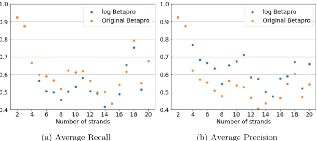
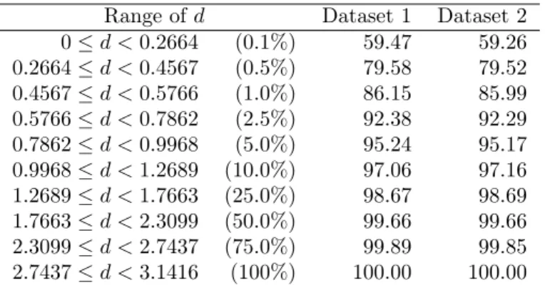
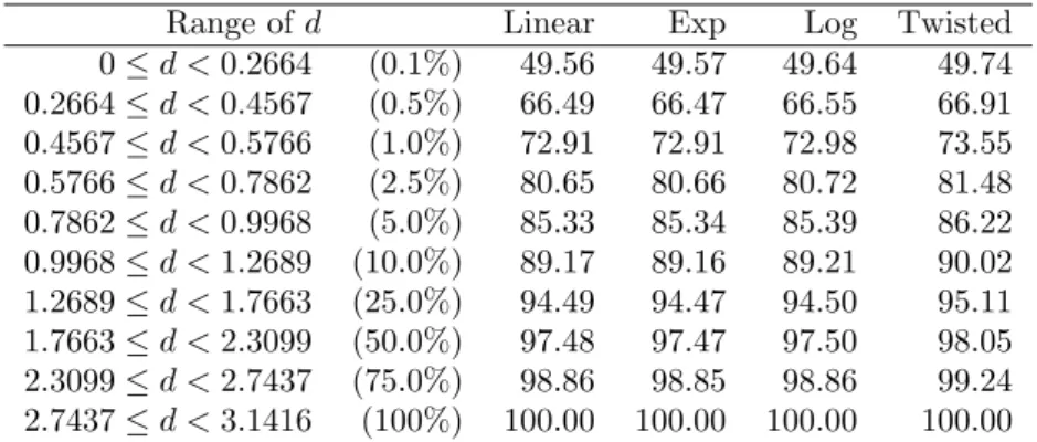
We also investigated the effect of different gap scores using the simplest substitution matrix; 1 along the diagonal (match) and -1 elsewhere (mismatch), with different gap scores. Perhaps surprisingly, the prediction accuracy using this simple substitution matrix was very similar to the result obtained using a large twist penalty (Table 22). There was a decrease in accuracy when the gap score was set to 0 and a relatively large improvement when it was set to -5.

Discussion

It is also possible that further development of the substitution matrix may improve prediction accuracy. 10] Andersen, Jørgen Ellegaard, Borot, Ga¨etan, Chekhov, Leonid O. and Orantin, Nicolas. ABCD topological recursion. We also show distributions of the same data, filtered by the number of leaves Figure B.2 and by the number of strands Figure B.3.