PhD Dissertation - Department of Mathematics

Another property of this class of models is the assumption regarding the conditional distributions of the answers given the random components. The parameters of this distribution can be derived using the predicted values ​​of the random components obtained by estimating each marginal model separately.

This class of models is combined with the theory of graphical models by deriving a graphical model based on the predicted values ​​of the random components under the model. In the paper we define a combination of two types of graphs that allow us to study the structure of dependence between random components and responses.

A multivariate model is constructed by assuming a multivariate Gaussian distribution, with zero expectation, of the random components representing the same tube in the six marginal models (the distributions of the different tubes are independent and identical). Using the extended separation theorem stated in Pelck & Labouriau (2021b), we were able to draw conclusions about the dependence structure of the responses based on the graphical model for the random components.

In addition, the random components representing the branches of study are assumed to be mutually independent. Furthermore, this result shows that the prediction of the random parts corresponding to the results in the entrance examination Mathematics is sufficient to predict the performance in Geometry.

Therefore, the result in the entrance exam in mathematics has a stronger influence on the performance in Geometry for this group of students. On the other hand, one can speculate whether the results in the entrance exam in Portuguese reflect the socio-economic class of the students which plays a key role in the performance in Geometry for the students who do not receive the bonus.

By combining the results of the undirected graphical model (UG) with the model assumptions, we construct a combination of a UG and a directed acyclic graph (DAG) to study how the dependency structure among the frailties affects the responses (Whittaker (1990) and Lauritzen (1996)). . The covariance structure of the random components (given by the covariance matrix Σ) will be characterized using the tools of graphical models.

Conditional Inference for Multivariate Generalised

Extended One Dimensional Generalised Linear Mixed Models

In Section I.2.2, we introduce an inference method involving predictions of the values ​​of the random components, B1,. Recall that the values ​​of the random components were predicted using equation (I.9), which is equivalent to solving the inference functions in (I.10) and (I.11).

Multivariate Models

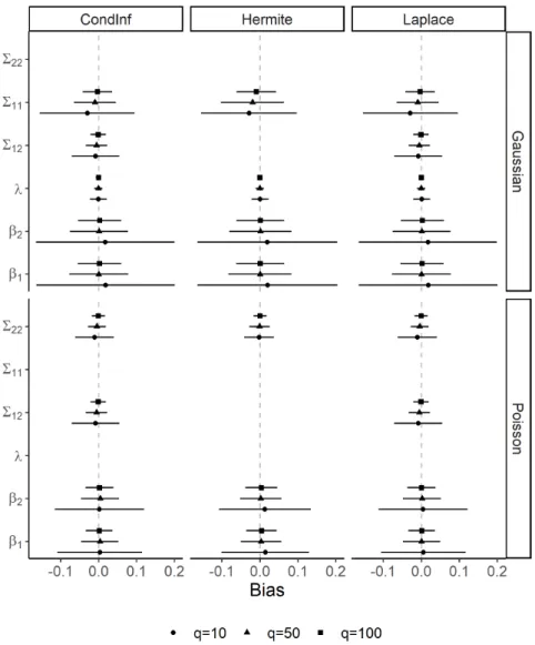
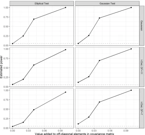
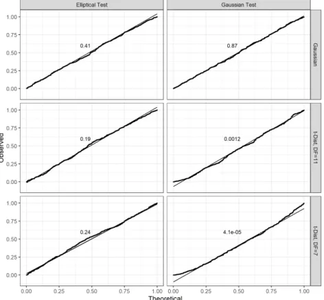
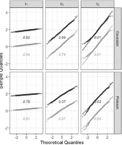
In the first simulation study, we simulate the model described above for three different covariance matrices, corresponding to three different values ​​of the constant in (I.14). In the second simulation study, we fix the covariance matrix of the random components to Σ defined in (I.14) with the constant set to one.

Discussion

2014), Information and exponential families: in statistical theory, John Wiley & Sons. 1993), 'Approximate inference in generalized linear mixed models', Journal of the American Statistics Association Mixed Models: Theory and Applications (Wiley Series in Probability and Statistics), Wiley-Interscience, USA. 2001), Multivariate statistical modeling based on generalized linear models, Springer-Verlag New York. 2012), Exponential Families and Theoretical Inference, Vol. 1996), 'Linear growth curve analysis based on exponential dispersion models', Journal of the Royal Statistical Society.

A Appendix

The method introduced involved a combination of multivariate generalized linear mixed models (GLMM) and graphical models to represent the covariance structure of the random components. In the analysis in this article, we focus on the analysis of the latent covariance structure of the random components.

Multivariate Generalised Linear Mixed Models With

Multivariate Generalised Linear Mixed Models

In this section, we formulate a version of the multivariate generalized linear mixed model described in Pelck & Labouriau (2021a). We define the density in terms of the Lebesgue measure of the elliptic contoured distribution by .

Representation of the Latent Covariance Structure via Graphical

For a consistent estimator of the covariance matrix or variance matrix, the distribution is only asymptotic. Under the model formulated in Section II.2.1, we can estimate the covariance matrix of the random components consistently based on consistent predictions of the random components by applying Proposition 1.

Discussion and Conclusion

Nevertheless, the assumptions on the distribution of the random components used here are weak and yield a flexible class of MGLMMs. Indeed, the test statistics of these tests depend only on the estimate of the covariance matrix.

A Appendix

Below we describe the covariance structure of the multivariate generalized linear mixed models we wish to introduce using two random components. For example, if the random variable V[Math] separates the random variable V[Geom] from the other points, then conditioning on only V[Math] makes V[Geom] independent of the other points (ie, V \nV[Geom] , V[Math]o).

Multivariate Generalised Linear Mixed Models for

Models for Scatter and Intensity of the Roots’ Colonisation

We model the spread at a fixed developmental stage by studying the occurrence of roots in the different observation windows of the minirhizotron tubes. According to Ramaley (1969), the length of a one-dimensional structure (the "noodle" replacing the needle) is proportional to the average number of times the structure crosses the reference lines.

Multivariate Simultaneous Models for the Scatter and the

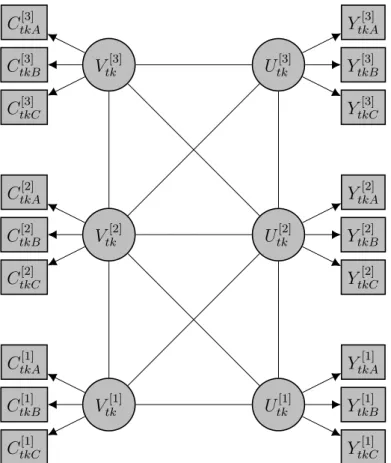
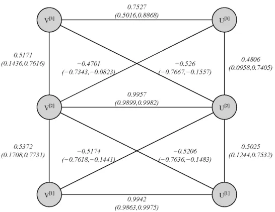
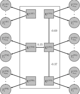
The interpretation of the graph above in terms of the random components of the multivariate generalized mixed model defined in Section III.3.1 is straightforward. The strength of this association can be estimated by deriving the entry of the precision matrix (i.e. Σ−1) corresponding to the random components U[1] and V[1].

Analysing the Motivational Example

In addition, we tested each of the possible vertices using the conditional test for random components under multivariate generalized linear mixed models described in Pelck & Labouriau (2021b). i.e. the variables in A) could continue the response variables in the third stage (i.e. the variables in B) is fully contained in the informational content contained in the random components associated with the second stage of development, and this conclusion holds for any combination of fertilization and depth zone. The graph was estimated by minimizing the BIC of a covariance selection model derived using the prediction of the random components.

Discussion and Conclusion

2020), 'Phosphorus in the profile of arable coarse sandy soils after 74 years with different applications of lime and p fertilizers', Geoderma Nitric oxide emissions and nitrogen use efficiency of manure and composted fertilizers applied to spring barley', Agriculture, Ecosystems and Environment Long-term effects liming and phosphorus application on the growth conditions of spring barley roots on sandy soil., Master's thesis, Aarhus University. 2021), Responses of spring barley root growth, mycorrhizal colonization and grain yield to long-term lime and phosphate application strategies on sandy soils. 2010), “Selecting high-dimensional mixed graphical models using AIC or BIC minimal forests”, BMC Bioinformatics Controlled traffic farming increased crop yield, root growth and nitrogen supply in two organic vegetable farms”, Soil and Tillage Research.

A Representation of the Covariance Structure in Terms of Direct

V[8] represents the individual variation in the ability of each of the n students that affects performance in the seven recordings. A more comprehensive description of the theory of graphical models can be found in Lauritzen (1996) and Whittaker (1990).

A Multivariate Methodology for Analysing Students’

Data Description

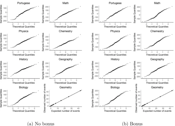
The first seven answers correspond to the student's performance in the university entrance exam in the disciplines: Mathematics, Physics, Chemistry, Biology, History, Geography and Portuguese. The last answer was the number of attempts students used to pass the geometry course (first year) at university.

A Multivariate Model for for Simultaneously Describing the

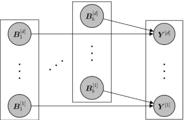
In each of two separate analyses, we used a multivariate model combining seven Gaussian mixed models describing the seven entrance exams and a discrete-time fragile Cox proportional model to model the number of attempts to pass the geometry course. We form marginal generalized linear mixed models for seven responses related to entrance exams by determining the conditional expectation of the random variable Yi[j] representing the ith individual (i= 1, . . . , n) in the jth dimension (j given ( Ue(i)[j] , Vi[j]) for j = 1,.

Modelling the Covariance Structure of the Random Components

V[8]} was derived using predicted values ​​of the random variables to derive a graphical model that minimizes the BIC. Note that this method only yields normally distributed predictors in cases with a small variation of the random components.

Results and Discussion

From a practical point of view, this result shows that the prediction of the random component V[Math] is sufficient to predict the performance of students who received bonus in geometry. We have another scenario for the population of students who did not receive a bonus.

A Some Model Control

2014), 'Multivariate survival mixed models for genetic analysis of longevity traits', Journal of Applied Statistics Student academic performance from inception to graduation through quasi u statistics: a study at a Brazilian research university', Journal of Applied Statistics Academic performance, the background of students and affirmative action at a Brazilian university', Higher education management and policy a), Conditional inference for multivariate generalized linear mixed models. where ti represents the observed time the student passes the course or is censored, and .

B Detailed Representation of the Graphical Models Involving the

We derive an undirected graphical model based on vulnerability predictions to study the covariance structure in the multivariate Gaussian distribution. Suppose the multivariate random components of the MGLMM have a covariance structure encoded by the graph G=(V, E).

A Multivariate Survival Model for Studying Time to

Data Description

We use a partial data from the project to study the cumulative emergence dynamics of annual weeds Scherner et al. 2017) to illustrate how the techniques in Pelck. The three operations used were: direct drilling (D), form board plow (P) to 20 cm soil depth and pre-sowing tine tillage (HW) to 8–10 cm soil depth (Scherner et al. 2017).

Multivariate Model

This was because they had shown very similar germination in the same experimental area and because it is difficult to differentiate them at an early stage of development (Scherner et al. 2017). That is, different physical locations in the field are independent for all responses, and the covariance structure within the same location is given by Σ.

Graphical Models

A key result in the theory of graphical models is that if a set of vertices, S, separates two disjoint subsets of vertices A and B, then all the variables in A are independent of the variables in B given the variables in S. In Pelck & Labouriau (2021b ) an extension of the separation principle called the induced separation principle is formulated.

Results and Discussion

The estimated conditional expectations given that propagules emerge before day T = 61 are shown in Figure V.2. In the fourth block, we see that the expected show times for the different treatments are very close.

A Appendix

The details of the construction are given in Section VI.3.1, and the graphical model representing the covariance structure of the random components is discussed in Section VI.3.2. We characterize the covariance structure of the MGLMM defined in Section VI.3.1 by defining a graphical model constructed with its arbitrary components.

Multivariate Methods for Detection of Rubbery Rot in

Models for Several Responses with Different Nature

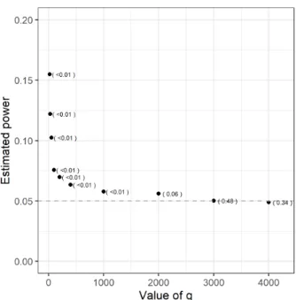
The probability of observing a zero value can be calculated as a function of the power index p and the expectation (see Jørgensen, 1987). This process was repeated for each value of the power index p in a grid of possible values.

Multivariate Simultaneous Models for Responses of Different

In the analysis described above, we calculated the probability that each observation takes the value zero using a grid of values ​​of the power index p. The following basic graph theory definitions will be needed to characterize the covariance structure of the MGLMM we are working with.

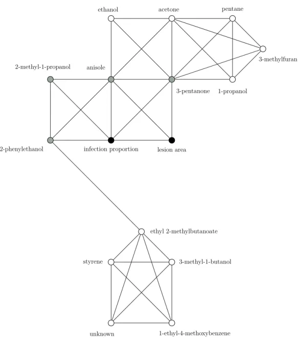
Results

This result implies that the knowledge of the random components in S makes the VOCs in ˜A uninformative with respect to the lesion area and the proportion of apples showing visible symptoms. We modeled the predicted values ​​of the random components of those models by finding the graph that minimizes the BIC (Bayesian Information Criterion) as exposed in Abreu et al.