C
2004Kluwer Academic Publishers. Printed in the Netherlands.
A Fractional Linear System View of the Fractional Brownian Motion
MANUEL DUARTE ORTIGUEIRA∗and ARNALDO GUIMAR ˜AES BATISTA
UNINOVA/DEE, Campus da FCT da UNL, Quinta da Torre, 2825 – 114 Monte da Caparica, Portugal;∗Author for
correspondence (e-mail: [email protected]; fax:+351-1-2957786) (Received: 28 November 2003; accepted: 15 March 2004)
Abstract. A definition of the fractional Brownian motion based on the fractional differintegrator characteristics is proposed and studied. It is shown that the model enjoys the usually required properties. A discrete-time version based in the backward difference and in the bilinear transformation is considered. Some results are presented.
Key words: backward difference, bilinear transformation, fractional Brownian motion, fractional differintegrator, Hurst parameter
1. Introduction
Fractional Brownian motion (fBm), 1/f noises, self-similaririty and long range dependence are inter-connected notions and appear in a variety of contexts [1–3]. The starting point was the introduction of the fBm by Mandelbrot and Van Ness [1, 2] as a model for non-stationary signals, but with stationary increments, that are useful in understanding phenomena with long range dependence and with a fre-quency dependence of the form 1/fα, withαnon-integer. The proposal of Mandelbrot and Van Ness
can be stated as follows:
Let H,0 < H < 1, be the called Hurst parameter and b0 a number. Then the fBm, BH(t), with
parameterHis defined by:
BH(t)−BH(0)=
1 Ŵ(H+1/2)
0
−∞
[(t−τ)H−1/2
−(−τ)H−1/2
]dB(τ)
+
t
0
(t−τ)H−1/2dB(τ)
(1)
whereBH(0)=b0, andB(t) is the standard Brownian motion.
Following a comon practice in engineering texts, we will introduce the stationary white noise process, w(t), instead ofdB(t). Although there are other definitions and approaches to fBm, the above definition is usually accepted. In this paper, we will look at the above definition and interpret it in terms of the fractional differintegrator, showing that it is unacceptable and propose a different approach in the line of thoughts followed in [4, 5]. As it is important to have a discrete-time version , not only for simulating the continuous-time case, but because there are a lot of applications that are essentially discrete-time, we will face the problem of defining a discrete-time fBm (see [6] for an alternative approach).
2. The Proposed fBm and Its Properties
We begin by rewriting the above definition in the format:
BH(t)−BH(0)=
1 Ŵ(H+1/2)
t
−∞
(t−τ)H−1/2w(τ)dτ −
0
−∞
(−τ)H−1/2w(τ)dτ
(2)
As it can be seen, the fBm as assumed by this definition is a strange signal because it is the difference of the values attand 0 of a signal defined as the output of a fractional integrator when the input is white noise:
BH(t)=
1 Ŵ(H+1/2)
t
−∞
(t−τ)H−1/2w(τ)dτ (3)
Besides this integrator has orderH+1/2 and, as 0<H <1, it is unstable, even in wide sense, for 1/2<H<1, the so-called persistent case. On the other hand, the autocorrelation function ofBH(t) is
easily computed and it is given by:
R(τ)=σ2 |τ|
2H
2Ŵ(2H+1) sinHπ (4)
whereσ2is the white noise variance. However, for the assumed interval forH, this function is not a
valid autocorrelation function, because it does not have a maximum at the origin. These considerations lead us, according to [4, 5], to propose the following approach to define fBm.
Let w(t) be a continuous-time stationary white noise with varianceσ2. We callαorder fractional noise, rα(t), the output of anα-order differintegrator,|α|<1, when the input is white noise, w(t):
rα(t)=
1 Ŵ(α)
t
−∞
w(τ)·(t−τ)α−1dτ (5)
where we putr0(t)= w(t). Ifw(t) is Gaussian, therα(t) is the so calledFractional Gaussian Noise
(FGN). The theory we present in this paper does not require thatw(t) be a Gaussian process; so we will not assume this.
The fractional noise,rα(t), is a wide sense stationary stochastic process with a autocorrelation
func-tion:
R(t)=σ2 |τ|
2α−1
2Ŵ(2α) cosαπ (6)
Although the signal has an infinite power, its mean is constant and the autocorrelation function E{rα(t+τ)·rα(t)}depends only ofτ, not oft. Relation (9) shows that we only have a (wide sense)
stationary hyperbolic noise if 0 < α < 1/2. The other cases do not lead to a valid autocorrelation function of a stationary stochastic process, since it does not have a maximum at the origin. The above-defined process is a somehow “strange” process with infinite power. However, the power inside any finite frequency band is always finite. Its spectrum is:
Sr(ω)=
σ2
|ω|2α (7)
We obtained a way of generating a fractional stationary process that can be used to define the fBm.
Let rα(t) be a continuous-time stationary hyperbolic noise. Define a processvα(t), t≥0, by:
vα(t)=
t
0
rα(τ)dτ (8)
If|α| <1/2 we will call this process a fractional Brownian motion (or generalised Wiener–L´evy process).
This is a generalisation of the ordinary Brownian noise that is obtained withα=0.
For the proof, we are going to show that it enjoys all the properties normally required for the fBm.
1. vα(0)=0 andE{vα(t)} =0 for everyt≥0(1)
2. The covariance is:
E[vα(t)vα(s)]=E
t
0
rα(τ)dτ
s
0
rα(t′)dτ′
= t 0 s o
E[rα(τ)rα(τ′)dτdτ′]
=σ2 1
2Ŵ(2α) cosαπ
t
0
s
0
|τ −τ′|2α−1dτdτ′
= σ
2
2Ŵ(2α+2) cosαπ[|t|
2α+1
+ |s|2α+1− |t−s|2α+1] (9)
PuttingH =α+1/2, we obtain the usual formulation:
E[vα(t)vα(s)]=
VH
2 [|t|
2H+ |s|2H− |t−s|2H] (10)
with
VH =
σ2
Ŵ(2H+1) sinHπ (11)
that is much more simple than the usual. The variance is readily obtained:
E[vα(t)2]=VH|t|2H (12)
3. The process has stationary increments.
We are going to show that the increments
vα(t,s)=vα(t)−vα(s)=
t
s
rα(τ)dτ (13)
are stationary. The computation of the variance is slightly involved. We have:
Var{vα(t,s)} =
t
s
rα(τ)dτ
t
s
rα(τ′)dτ′
= t s t s
E[rα(τ)rα(τ′)]dτdτ′
Using Equation (9), we obtain:
Var{vα(t,s)} =σ2
1 2Ŵ(2α) cosαπ
t
s
·
t
s
|τ −τ′|2α−1dτdτ′ (14)
1Ifw(t) is Gaussian, so it isr
As the primitive of|u|αis |u|α+1
α+1·sgn(u), where sgn(·) is the signum function, it is a simple matter to
prove that:
Var{vα(t,s)} =σ2
|t−s|2α+1
2Ŵ(2α+2) cosαπ (15)
This result confirms that the increments are stationary. In particular, witht =s+T, we obtain:
Var{vα(s+T,s)} =σ2
T2α+1
2Ŵ(2α+2) cosαπ (16)
and
Var{vα(s+T,s)} =σ2
T2H
2Ŵ(2H+1) sinHπ (17)
as in [2] by puttingH =α+1/2; asα∈]−1/2,1/2[,H∈]0, 1[. With these values forH, we are confirming the considerations done by Mandelbrot and Ness. These results are also in agreement with the theory and results developed by Reed et al. [4]. We must remark that, contrary to the ordinary Brownian motion,vα(t) does not have independent increments.
4. The process is self similar In fact, from (10), we have:
E[vα(at)vα(as)]=
VH
2 [|a·t|
2H+ |a·s· |2H− |a·t−a·s|2H
]
= VH
2 |a|
2H
[|t|2H+ |s|2H− |t−s|2H] (18)
that shows that the process is self-similar. 5. The incremental process has a 1/fβ spectrum
Defining an incremental process by:
dH(t)=vH(t)−vH(t−T) (19)
we conclude that its autocorrelation function of the incremental process is
Rd(τ)=
VH
2 [|τ +T|
2H+ |τ−T|2H−2|τ|2H] (20)
and, as [10]
FT
1
2Ŵ(β) cos(βπ/2)|t|
β−1
= 1
|ω|β (21)
the corresponding spectrum of the incremental process is given by:
Sd(ω)=σ2.
sin2(ωT/2)
|ω|2H+1 (22)
6. The autocorrelation function of sampled version of the incremental process
dH(n)=vα(nT)−vα[(n−1)T] (23)
whereT is the sample interval given by:
Rdis(k)= VHT
2 [|k+1|
2H+ |k−
1|2H−2|k|2H] (24)
and the corresponding spectrum is given by the Polya’s summation formula [7]:
Sdis(ω)=σ2sin2(ωT/2)
+∞
n=−∞
1 ω+2π
T n
IfT is enough low,T <<π, we have:
Sdis(ω)≈σ2sin2(ωT/2) 1
|ω|2H+1 |ω|< π/T (26)
and, for lowω, ω→0, we obtain:
Sdis(ω)≈σ2(T/2)2 1
|ω|2H−1 (27)
This means that asymptotically, the autocorrelation must be proportional to|k|2H−2. In fact, from
(24), we obtain
Rdis(k)= VHT
2 |k|
2H
[|1+1/k|2H+ |1−1/k|2H−2] (28)
and, using the binomial expansion:
Rdis(k)= VHT
2 |k|
2H ∞
i=1
2H
2i |k|
−2i (29)
where
2H
2i =
(−1)2i(−α) 2i
(2i)!
are the binomial coefficients. If|k|is very high, we have:
Rdis(k)≈ VHT
2 |k|
2H−2
(30)
as affirmed above.
Results (25) to (27) show something interesting [1, 2]:
7. If 1/2<H <1, the spectrum has a hyperbolic character, corresponding to a persistent fBm, because the increments tend to have the same sign;
8. If 0 < H <1/2, the spectrum is parabolic, corresponding to an antipersistent fBm, because the increments tend to have opposite signs.
3. A Discrete-Time Fractional Noise
In the discrete-time case, the problem is in the definition of a discrete-time fractional noise (dFN), e.g. the discrete-time version of Equation (8). The common approach to model the fractional noise is based on the backward difference conversion [9] that can be considered as a discretization of the Gr¨unwald-Letnikov fractional derivative [5, 8]. However, according to the theory we presented in section 2, this may be incorrect in the persistent case. As it is well known, (1−e−jω) (2) is the frequency response of the
usual discrete-time approximation for the continuous-time derivative (jω), but its inverse, 1/1−e−jω
, is not a good approximation to 1/jω. For this, we prefer the bilinear transformation 1/+e−jω/1−e−jω.
This means that we can use different definitions for the discrete-time fractional noise, depending on the used approximation: backward, bilinear or other. According to what we said above, we define a discrete-time fractional noise as the white noise driven output of a discrete-time system with transfer function given by:
(a) Hbd(z)=(1−z−1)1/2−H, |z|>1 (31)
or, by
(b) Hbil(z)=
2·1−z
−1
1+z−1 1/2−H
|z|>1 (32)
If 0< H <1/2 we obtain fractional differentiators, while if 1/2< H <1, we obtain integrators. The corresponding spectra are easily computed, provided that we use:
S(ejω)=σ2· lim
z→ejωH(z)·H(z
−1
) (33)
They are given by:
Sbd(ejω
)=σ2·21−2H[sin(ω/2)]1−2H (34)
and
Sp(ejω)σ2·21−2H
sin(ω/2) cos(ω/2)
1−2H
(35)
Forω→0 and attending to the facts that cos(ω/2)≈1 and sin(ω/2)≈ω/2, we obtain:
Sp(ejω)=Sa(ejω)≈σ2·
1
|ω|2H−1
in agreement with (27). This means that, asymptotically, both the autocorrelation functions behave like
|k|2H−2agreeing with (30).
The computation of the inverse Z Transform of (32) (impulse response) is simple by using the binomial series expansion:
Hbd(n)=
1/2−H n (−1)
nu n=
(H−1/2) n!
nu
n (36)
whereunis the discrete-time Heaviside function and (a)n =a(a+1). . .(a+n−1) is the Pochhammer
symbol. Concerning to (33), we can say that the corresponding impulse response is a convolution of two binomial sequences corresponding to the numerator and denominator. However, it is not difficult to obtain:
hbil(n)=21−2H
n
k=0
(H−1/2)k
k!
(−1)n−k(1/2−H) n−k
(n−k)!
As
n!=(−1)k(−n)k(n−k)! k≤n (37)
and
we obtain:
hbil(n)=21−2H(−1)
n(1/2−H) n
n!
n
k=0
(H−1/2)k(−n)k
(H−1/2−n+1)k
(−1)k
k!
=21−2H(−1)
n(1/2−H) n
n! 2F1(H−1/2,−n;H−1/2−n+1;−1) (39)
where2F1(a, b; c, 1) is the Gauss hypergeometric function.
The autocorrelation function corresponding to (32) is not very difficult to compute and it is given by [10]:
Rbd(k)=σ222−4H(−1)k Ŵ(2−2H)
Ŵ(3/2−H+k)Ŵ(3/2−H−k) (40)
With some work and using the properties of the Gamma function, we can prove the asymptotic behaviour stated before. Relatively to the bilinear case, it seems that there is no closed formula for its autocorrelation function. It is essentially the autocorrelation of (39). It can also be expressed as the convolution of two sequences like (40).
4. Simulation Results
To test the ability of the above ways of generating the dFN, we made some simulations in the following way. For each method:
We computed a long impulse responseL =2000 in the backward difference andL =4000 in the bilinear case (this is due to the fact that the impulse response is a convolution of two backward like impulse responses).
We generated 100 sequences with lengthL+M. We discarded the firstLvalues. With theMvalues we estimated the Hurst parameter.
We computed the mean and variance of each parameter estimate.
There are several estimation procedures for obtaining the Hurst parameter [11–13]: (a) Aggregated variance method
(b) Absolute values of the aggregated series (c) Higuchi’s method
(d) Residuals of regression (e) The R/S method (f) Periodogram method (g) Whittle estimator (h) Abry-Veitch
(i) AR method
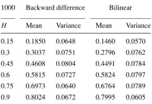
Here we adopted the aggregated variance method for its simplicity. In the following table, we present the results forM=1000 andM =2000.
As it can be seen, both the algorithms perform poorly in the integral case (H >1/2) and with some surprise we see that the bilinear conversion is slightly better even in the derivative case (H <1/2).
Table 1. Estimation of the Hurst parameter using 1000 points and the aggregated variance method.
1000 Backward difference Bilinear
H Mean Variance Mean Variance 0.15 0.1850 0.0648 0.1460 0.0570 0.3 0.3037 0.0751 0.2796 0.0762 0.45 0.4608 0.0804 0.4491 0.0784 0.6 0.5815 0.0727 0.5824 0.0797 0.75 0.6973 0.0640 0.6764 0.0789 0.9 0.8024 0.0672 0.7995 0.0605
Table 2. Estimation of the Hurst parameter using 2000 points and the aggregated variance method.
2000 Backward difference Bilinear
H Mean Variance Mean Variance 0.15 0.1908 0.0457 0.1600 0.0490 0.3 0.3122 0.0517 0.3081 0.0491 0.45 0.4448 0.0504 0.4379 0.0523 0.6 0.5809 0.0594 0.5902 0.0541 0.75 0.7118 0.0493 0.7180 0.0514 0.9 0.8239 0.0466 0.8287 0.0458
5. Conclusions
In this paper, we made a brief approach into the fractional Brownian motion definition taking as starting point the definition of fractional continuous-time linear system. We performed an analysis of the definition proposed by Mandelbrot and van Ness and showed why it is unsatisfactory. An alternative approach was proposed based on the fractional differintegrator. We defined the fractional Brownian motion as an integral of a fractional noise defined as the output of a differintegrator when the input is white noise. We studied approaches based on the backward difference and bilinear transformations to define the discrete-time approximations to the differintegrator. Some illustrating simulation results showed that the bilinear based differintegrator is slightly better.
References
1. Mandelbrot, B. B.,The Fractal Geometry of Nature, W. H. Freeman, New York, 1983.
2. Mandelbrot, B. B. and Van Ness, J. W., ‘The fractional Brownian motions, fractional noises and applications’,SIAM Review
10(6), 1968, 422–437.
3. Keshner, M. S. ‘1/f Noise’,Proceedings of IEEE70, March 1982, 212–218.
4. Reed, I. S., Lee, P. C., and Truong, T. K., ‘Spectral representation of fractional Brownian motion inndimensions and its properties’,IEEE Transactions on Information Theory41(8),1995, 1439–1451.
5. Ortigueira, M. D. ‘Introduction to fractional signal processing. Part 1: Continuous-time systems’,IEE Proceedings on Vision, Image and Signal Processing1, February 2000, 62–70.
6. Li, M. and Chi, C-H., ‘A correlation-based computational model for synthesizing long-range dependent data’,Journal of the Franklin Institute340,2003, 503–514.
8. Samko, S. G., Kilbas, A. A., and Marichev, O. I.,Fractional Integrals and Derivatives - Theory and Applications,Gordon and Breach, Amsterdam, 1993.
9. Hosking, J., ‘Fractional differencing’,Biometrika68, 1981, 165–176.
10. Ortigueira, M. D., ‘Introduction to fractional signal processing. Part 2: Discrete-time systems’,IEE Proceedings on Vision, Image and Signal Processing1, February 2000, 71–78.
11. Taqqu, M. S., Teverovsky, V., and Willinger, W., ‘Estimators for long-range dependence: an empirical study’,Fractals3(4), 1995, 785–788.
12. Karagiannis, T., Faloutsos, M., and Riedi, R. H., ‘Long-range dependence: Now you see it, now, you don’t!’, inProceedings Global Internet, Taiwan, November 2002.