Universidade Federal de Minas Gerais Instituto de Ciˆencias Exatas
Departamento de Ciˆencia da Computac¸ ˜ao
Navega¸
c˜
ao e Controle de Robˆ
os M´
oveis Cooperativos:
Uma Abordagem baseada em Conectividade de Grafos
Guilherme Augusto Silva Pereira
Tese apresentada ao Curso de P´os-Gradua¸c˜ao em Ciˆencia Computa¸c˜ao da Universidade Federal de Minas Gerais como requisito parcial para obten¸c˜ao do t´ıtulo de Doutor em Ciˆencia da Computa¸c˜ao.
Orientador: Prof. M´ario Fernando Montenegro Campos Co-orientador: Prof. Vijay Kumar
Universidade Federal de Minas Gerais Instituto de Ciˆencias Exatas
Departamento de Ciˆencia da Computac¸ ˜ao
Motion Planning and Control of Cooperating Mobile
Robots: A Graph Connectivity Approach
Guilherme Augusto Silva Pereira
Thesis presented to the Graduate Program in Computer Science of the Federal University of Minas Gerais in partial fulfillment of the requirements for the degree of Doctor in Computer Science.
Advisor: Prof. M´ario Fernando Montenegro Campos Co-Advisor: Prof. Vijay Kumar
To Cinthia,
the love of my life.
Resumo
Esta tese aborda o problema de navega¸c˜ao e controle de grupos de robˆos
m´oveis cooperativos. ´E proposta uma metodologia geral baseada em
conecti-vidade de grafos que fornece uma ´unica solu¸c˜ao para v´arias tarefas
coopera-tivas. A metodologia, que se baseia na redu¸c˜ao de v´arias tarefas cooperativas
em um problema b´asico ´unico, possibilita um mesmo time de robˆos m´oveis
executar diversas tarefas com um ´unico conjunto de algoritmos
parametriza-dos pelas caracter´ısticas de cada tarefa. Assim, mesmo uma tarefa totalmente
nova e desconhecida poderia ser realizada se esta pudesse ser transformada
em uma tarefa j´a conhecida pelos robˆos. A chave ´e a transforma¸c˜ao de
ta-refas cooperativas em m´ultiplos problemas individuais de planejamento de
movimento restrito. Para tal, um grupo de robˆos ´e modelado como um
grafo, onde cada robˆo ´e um v´ertice e cada aresta representa uma restri¸c˜ao
de movimento imposta por outros robˆos do grupo e que variam de acordo
com a tarefa. Em geral, estas restri¸c˜oes podem ser utilizadas em simples
e bem conhecidas t´ecnicas de navega¸c˜ao e controle para um ´unico robˆo. A
t´ecnica explorada neste texto ´e totalmente descentralizada e seus algoritmos
s˜ao baseados na modifica¸c˜ao em tempo real de fun¸c˜oes de navega¸c˜ao
especifi-cadas a priori. Para validar a metodologia, s˜ao mostrados exemplos pr´aticos
em sensoriamento colaborativo, comunica¸c˜ao e manipula¸c˜ao, todos avaliados
experimentalmente com grupos de robˆos holonomicos e n˜ao-holonomicos.
Abstract
This thesis addresses the problem of motion planning and control of
groups of autonomous mobile robots during cooperative tasks execution. A
general framework that transforms several cooperative tasks into the same
basic problem is developed thus providing a feasible solution for all of them.
The approach enables using a single team of robots to perform numerous
different tasks by providing each robot in the team with a single suite of
algorithms which are parameterized by the specificities of the tasks.
There-fore, even a totally new and unknown task can be executed by the group
of robots if this particular task can be transformed to one of the tasks the
team is able to execute. The key is the transformation of cooperative
prob-lems to individual constrained motion planning probprob-lems. In order to do
so, the group of robots is modeled as a graph where each robot is a vertex
and each edge represents a motion constraint to be satisfied. Motion
con-straints are imposed by the task and by the other robots in the group. These
constraints may be used in simple and very well known motion planning
tech-niques in order to plan and control the motion of each individual robot. We
present a decentralized solution for the problem, which algorithms are based
on the online modification of pre-specified navigation functions. Examples in
sensing, communication and manipulation tasks are presented, eliciting the
elegance of the solutions. Finally, experimental results with groups of both
non-holonomic and holonomic robots are presented.
Agradecimentos
Esta tese n˜ao teria sido conclu´ıda sem a ajuda de pessoas muito
impor-tantes e queridas.
Gostaria de agradecer `a toda minha familia pelo apoio incondicional
du-rante toda a minha vida. Sem eles eu n˜ao teria chegado at´e aqui.
Sou imensamente grato a minha querida esposa Cinthia pelo
companhei-rismo, amizade e amor. Esta tese certamente n˜ao seria poss´ıvel sem ela.
Agrade¸co ao Professor Mario Campos pelo apoio, amizade e confian¸ca
demonstrados em todos estes anos de conv´ıvio. Muitas vezes ele apostava
mais em mim do que eu mesmo o faria. Serei eternamente grato pelas diversas
oportunidades que ele me proporcionou.
O Professor Vijay Kumar foi de extrema importˆancia, n˜ao s´o para
ela-bora¸c˜ao deste trabalho, mas principalmente para o meu amadurecimento
como pesquisador. A nossa curta convivˆencia certamente influenciar´a toda a
minha vida cient´ıfica. Agrade¸co-o imensamente pela paciˆencia ao ler minhas
muito mal tra¸cadas linhas e ouvir minhas n˜ao t˜ao claras id´eias.
Gostaria tamb´em de agradecer aos demais membros da minha banca,
professores Luis Antˆonio Aguirre, Renato Cardoso Mesquita, Teodiano
Bas-tos Filho e Jos´e Reginaldo Hughes Carvalho, pelas opini˜oes e sugest˜oes de
melhoria do trabalho. Gostaria ainda de ressaltar a participa¸c˜ao dos
pro-fessores Luis Aguirre e Renato Mesquita na minha forma¸c˜ao profissional, j´a
que como professores de gradua¸c˜ao e p´os-gradua¸c˜ao, n˜ao s´o me forneceram
viii AGRADECIMENTOS
embasamento te´orico e pr´atico, como tamb´em me inspiraram a ingressar na
carreira cient´ıfica e acadˆemica.
Agrade¸co aos colegas Aveek Das, John Spletzer, Dan Gomez-Ibanez, e
Dan Walker pela ajuda com os robˆos, software e experimentos no GRASP
Lab. Al´em destes gostaria de lembrar o amigo Rahul Rao, por tornar a vida
longe de casa menos dif´ıcil.
Meu muito obrigado a todos os colegas do VERLab pelo ´otimo ambiente
de trabalho, em especial Bruno, Samuel, Denilson, Andr´ea, Pedro, Fl´avio,
Jo˜ao e Pio. Um agradecimento muito especial aos colegas Fernanda e Sancho,
pela ajuda com os robˆos holonˆomicos, Pinheiro, pela grande ajuda com as
“burocracias acadˆemicas”, e Wilton, que foi o grande respons´avel pela
“tele-presen¸ca” do Prof. Kumar durante a defesa da tese.
Um agradecimento especial a Luciana e Chaimo pela grande ajuda na
transi¸c˜ao BH/Philly. Sua amizade foi ainda fundamental para amenizar a
saudade de casa.
Merecem ainda meus agradecimentos todos os funcion´arios do DCC e do
GRASP, em especial Renata e Emilia, que sempre resolveram com prontid˜ao
toda a burocracia associada ao processo de doutoramento, e Dawn Kelly e
Genny Prechtel, pela ajuda burocr´atica na UPENN.
Agrade¸co ao CNPq pelo suporte financeiro.
Finalmente, agrade¸co a todos aqueles com quem tive a oportunidade de
conviver e trabalhar e que participaram direta ou indiretamente do processo
Acknowledgments
This thesis would not be concluded without the support of very important
and special people.
I would like to thank my family for the unconditional support during my
whole life. Without them I would never get this far.
I’m very grateful to my beloved wife Cinthia for her support, friendship
and love. This thesis would not be possible without her.
Thanks to Professor Mario Campos for his support, friendship and
trusti-ness in all these years we have been working together. Many times he had
more faith in me than I did myself. I will be eternally grateful for the various
opportunities he has presented me.
Professor Vijay Kumar was extremely important, not only for the
con-clusion of this thesis, but also for my development as a researcher. The short
time we have worked together will certainly influence my whole scientific life.
I thank him very much for his patience in reading my poorly written words
and listening to my not so clear ideas.
I would like to thank the other members of my thesis committee,
profes-sors Luis Antˆonio Aguirre, Renato Cardoso Mesquita, Teodiano Bastos Filho
and Jos´e Reginaldo Hughes Carvalho, for their opinions and suggestions to
improve this work. Also, I would like to mention the influence professors Luis
Aguirre and Renato Mesquita had in my professional life. As
undergradu-ate and graduundergradu-ate professors they not only gave me theoretical and practical
x ACKNOWLEDGMENTS
background, but also inspired me to choose the scientific and academic career.
I thank Aveek Das, John Spletzer, Dan Gomez-Ibanez, and Dan Walker
for helping with robots, software and experiments at the GRASP Lab. Also,
I would like to thank my officemate and friend Rahul Rao for making life far
from home less difficult.
Many thanks to my fellow students at VERLab for creating an enjoyable
working environment and in special to Bruno, Samuel, Denilson, Andr´ea,
Pedro, Fl´avio, Jo˜ao and Pio. Special thanks to Fernanda and Sancho, for
helping with the holonomic robots, to Pinheiro, for helping with the
“aca-demic bureaucracy”, and to Wilton, the main responsible for the “virtual
presence” of Prof. Kumar during the thesis defense.
Special thanks to Luciana and Chaimo for the enormous help in the
tran-sition BH/Philly. Their friendship was also essential to ease our homesick.
Also deserve my gratitude, the staff of DCC and GRASP, in special
Re-nata and Emilia, for solving promptly all bureaucracy associated with the
doctorate program, and Dawn Kelly and Genny Prechtel, for helping with
the paperwork in GRASP.
I thank CNPq for the financial support.
Finally, I thank all people with whom I’ve had the opportunity to work
with, and who participated directly or indirectly in this work. Thank you
Contents
List of Figures xiv
List of Tables xxi
List of Symbols xxiii
1 Introduction 1
1.1 Motivation . . . 2
1.2 Approach . . . 4
1.3 Contributions . . . 6
1.4 Organization . . . 7
2 Related Work 9 2.1 Multi-Robot motion coordination . . . 10
2.2 Cooperative Manipulation . . . 13
2.3 Communication in Robot Teams . . . 14
2.4 Multi-Robot Sensing . . . 17
3 Background 21 3.1 World Modeling . . . 21
3.2 Transformations and Lie Groups . . . 23
3.3 Configuration Spaces . . . 25
3.4 Sets . . . 27
3.5 Robot Motion Planning . . . 29
3.6 Motion Constraints . . . 33
3.7 Lyapunov Stability . . . 35
3.8 Graphs . . . 37
4 Motion Planning with Cooperative Constraints 41 4.1 Problem Definition . . . 41
4.2 Motion Planning Approach . . . 43
4.2.1 Neighborhood Relationships . . . 44
xii CONTENTS
4.2.2 Decentralized Controllers . . . 49
4.3 Extension to Real Robots . . . 57
4.3.1 Non-Holonomic Robots . . . 58
5 Application to Sensing and Communication 61 5.1 Introduction . . . 61
5.2 Sensing and Communication Networks . . . 63
5.2.1 Formation Constraints . . . 64
5.3 Planning and Control . . . 65
5.4 Experimental Results . . . 68
5.4.1 Non-holonomic robots . . . 68
5.4.2 Holonomic robots . . . 72
5.5 Concluding Remarks . . . 78
6 Application to Manipulation 81 6.1 Introduction . . . 81
6.2 Object Closure . . . 84
6.2.1 Definition . . . 84
6.2.2 A Test for Object Closure . . . 87
6.2.3 Introducing Rotations . . . 89
6.2.4 Polygonal Robots . . . 90
6.2.5 Circular Robots and Objects . . . 92
6.3 Planning and Control . . . 94
6.4 Experimental Results . . . 97
6.5 Concluding Remarks . . . 100
7 Application to Formation Control 103 7.1 Introduction . . . 103
7.2 Problem definition . . . 105
7.3 Potential Functions . . . 107
7.4 Controllers . . . 109
7.5 Experimental Results . . . 113
7.6 Concluding Remarks . . . 115
8 Conclusions and Future Work 119 8.1 Summary . . . 119
8.2 Future Work . . . 123
CONTENTS xiii
A Multi-Robot Platforms 137
A.1 GRASP Lab. Platform . . . 137
A.1.1 Vision system . . . 139
A.2 VERLab Platform . . . 144
B Collaborative Localization and Tracking 147 B.1 Introduction . . . 147
B.2 Mathematical Modeling . . . 148
B.3 Measurements Transformation . . . 149
B.4 Measurements Combination . . . 153
B.4.1 Dynamical Systems . . . 156
B.5 Localization Approach . . . 157
B.5.1 Centralized × Distributed . . . 162
B.5.2 Global Localization . . . 163
B.6 Experimental Results . . . 163
List of Figures
1.1 Two robots in a disaster situation. . . 3
1.2 Two robots in tightly coupled cooperation carrying a relative large box. . . 5
2.1 Four technics of manipulation: (a) force closure (robots press-ing the object); (b) form closure; (c) conditional closure (robots pushing the object up); (d) object closure or caging. . . 14
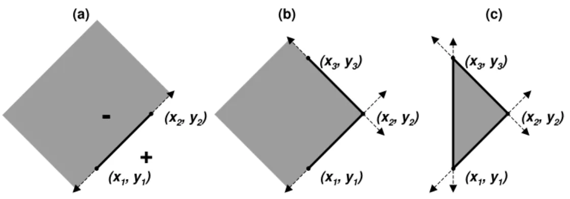
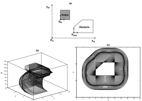
3.1 A convex polygonal entity can be represented by the intersec-tion of planes. (a) – Each edge equaintersec-tion divides the plane into two half planes. (b) and (c) – a triangular region is formed by the intersection of three half planes. . . 23 3.2 (a) – A polygonal robot and an obstacle; (b) – The
represen-tation of the obstacle in the configuration space (Cobs i); (c) –
The top view ofCobs i . . . 26
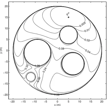
3.3 Equipotential contours of a navigation function in a circular environment with four circular obstacles. . . 32
3.4 Non-holonomic constraint: The position of the car in the plane is describe by three coordinates, but its velocity can only be along the vectorv. Thus, the changing rate of the three posi-tion coordinates is constrained. . . 34 3.5 Hamiltonian Graph as a common spanning subgraph of two
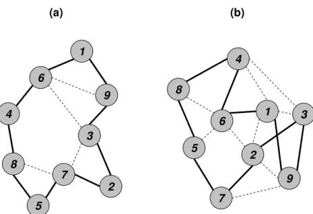
different graphs. The continuous edges represent the edges of the HGwhile the dashed ones are the other edges of the graph. 39
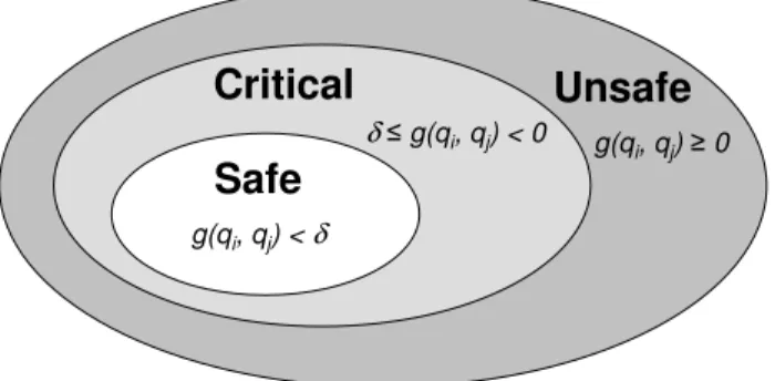
4.1 The activation of the constraints define three regions in the robots’ configuration space. . . 48 4.2 Switched control system with three modes. . . 50
xvi LIST OF FIGURES
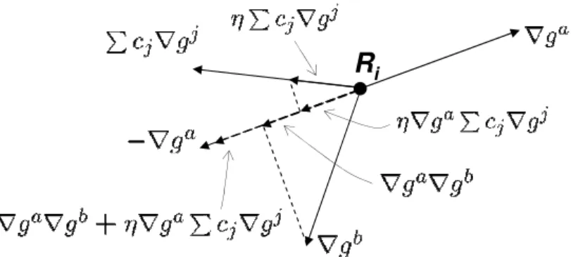
4.3 η is chosen in order to avoid Ri to move in a direction
con-trary to ∇ga and ∇gb. Only the constraint relative to ∇ga is
illustrated by simplicity. Observe that a small η was chosen such that ∇ga∇gb +η∇gaP
cj∇hj <−∇ga . . . 52
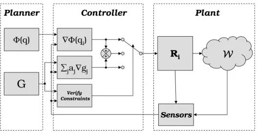
4.4 Block diagram of the system. . . 53 4.5 A non-holonomic robot. . . 59
5.1 Formation constraints: Rk induces constraints on the position
ofRi. IfRi is inside the circle defined byg ≤δ1 (outer dashed
circle), connectivity with Rk is guaranteed. The gray area
defined by g > δ3 and g < δ2 is asafe configuration space for
Ri, where collisions are avoided and connectivity is maintained. 65
5.2 Sensing graph for the experiment in Figure 5.3. . . 69 5.3 Three robots following their navigation functions while
main-tain sensing constraints with at least another robot. Ground truth data (trailing solid lines behind each robot) is overlaid on the equipotential contours of the navigation function for R3. 70
5.4 Sensing graph for the experiment in Figure 5.5. The gray
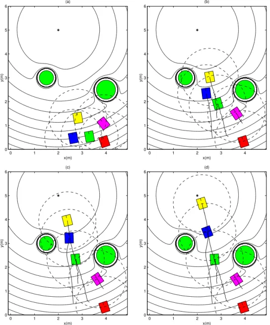
vertex is a static robot. . . 71 5.5 Deploying a mobile sensor network with five nodes. Figures
(a)–(d) show four snapshots of the same experiment. One of the robots is static and is considered a base. Ground truth data is overlaid on the equipotential contours of the navigation function for the robots. . . 71 5.6 Three holonomic circular robots flocking from initial
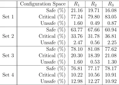
configu-rations to a target region avoiding a single circular obstacle. The dashed lines represent both the collision and the maxi-mum distance constraints. . . 73 5.7 Constraint graph for the experiment in Figure 5.6. . . 74 5.8 The four different sets of values forδ used in the experiments.
The dashed lines delimit valid configuration space represented by g(qi, qj)<0, and the continuous lines represent g(qi, qj) =
δ. The shadowed dark areas represent the safe regions of the configuration space and the shadowed light regions are the critical configuration spaces. (a) – Set 1, (b) – Set 2, (c) – Set 3, and (d) – Set 4. . . 74 5.9 Effect of δ in the mean time the robots spend in each region
LIST OF FIGURES xvii
5.10 This figure shows the same results in Figure 5.9 but now crit-ical and unsafe spaces were divided in two groups: (i) close – relative to the concave, avoidance constraint, and (ii) far – relative to the convex, maximum distance constraint. . . 78
6.1 Three approaches for caging. (a) – the object is able to rotate and, independently of its orientation, it cannot be removed from the robot formation; (b)– the object’s rotation is re-stricted. Caging is achieved for all possible orientations. The dashed objects represent the maximum and minimal orienta-tions; (c) –Object closure, the object is able to rotate. Closure is only guaranteed for a small set of orientations. The dashed object represents an example where the object can scape with a series of rotations and translations. Our approach is based on the fact that the object cannot execute movements like this one in small periods of time. . . 83 6.2 Cobj i for a point robot considering only object translations.
By sliding the object around the robot, the origin, o, of the object-fixed reference frame traces out the boundaries of Cobj i. 85
6.3 Object closure: the interior (shaded gray) represents the clo-sure configuration space, Ccls, for a team of 4 robots. The
dashed polygon represents the object. Notice that the origin of the object’s reference frame is inside Ccls, a compact set,
indicating a condition of object closure. . . 86 6.4 Essential Robots: even with the removal of R3 the closure
properties of the group are preserved and so, R3 is a
non-essential robot. . . 86 6.5 Object closure is achieved if each robot i is inside Γi. The
shaded areas represent (a)I1 and (b) Γ1. . . 89
6.6 Closure region for a maximum rotation of 20◦
. . . 90 6.7 Robot k checks closure (a) using the imaginary point robots,
Ri and Ri−1 (left) (b) using a different set of point robots, Ri and Ri+1 (right). The dotted polygons are the actual object
configuration space. . . 91 6.8 Three robots caging a triangular object. R1’s computation of
Cobj1 and Cobj2 for the imaginary point robots located at the
xviii LIST OF FIGURES
6.9 Object transportation: t1 – R2 and R3 are in the Achieve
mode (see Figure 4.2, page 50) trying to achieve object closure;
t2 – Object closure constraints are satisfied,R2 and R3 are in
the Maintain mode; t3 – The robots are in theGoToGoal
mode. R1 is in the GoToGoal mode in all three snapshots. . 99
6.10 The actual COBJ i (dashed polygons) for each robot. The
ori-gin of the object (◦) is always inside Ccls (the compact set
delimited by the three Cobj i) indicating an object closure
con-dition. (a) – initial and final configurations; (b) – an interme-diate configuration. . . 100 6.11 Test for object closure when the object (in this case another
robot) has a circular shape. An overlap between Cobj1 and
Cobj2 of the imaginary point robots at R1 and R2 indicates
that the circular robot cannot scape using this space. The same test for R2 and R3 indicates that the robot can scape
through this space. . . 101 6.12 Four robots caging a circular holonomic robot. Four snapshots
of the experiment are shown from left to right, and top to bottom. . . 102
7.1 Graph modeling for a group of 5 robots: (a) – formation con-trol graph; (b) – constraint graph. . . 105
7.2 A formation graph based on the combination of the graphs
of Figure 7.1. Based on incoming edges, R5 has configuration
space constraints on its position relative to R4, R1 follows a
potential function to acquire a position relative to R3, while
R2, R3, and R4 must execute a combination of two reactive
behaviors. . . 111 7.3 (a) – The control graph and (b) – the constraint graph for the
first experiment. . . 113 7.4 Four snapshots of an experiment where three robots are in line
formation and keeping visibility constraints with their follow-ers. The goal configuration for the lead robot is marked with a (*). The dashed circumferences represent the sensors’ field of view. In (c) robot R3 was manually stopped for 7 seconds.
The robots stop following their potential functions and wait for R3 so that the constraints are preserved. . . 114
7.5 The y coordinate for the experiment in Figure 7.4. The ter-minal follower, R3, was stopped for approximately 7 s at the
time 15 s. It causes the other robots to switch to theirUnsafe
LIST OF FIGURES xix
7.6 (a) – The control graph and (b) – the constraint graph for the second experiment. . . 116 7.7 Four snapshots of an experiment where three holonomic robots
are in a triangular formation. The goal configuration for the lead robot is marked with a (*). The dashed circumferences represent the boundaries of the valid configuration space. In (c) robot R3 was stopped. The lead robot (R1) stop
follow-ing its navigation function, waitfollow-ing for R3 causing its other
follower,R2, to stop as well. . . 117
7.8 The y coordinate for the experiment in Figure 7.7. The ter-minal follower, R3, was stopped for approximately 8 s at the
time 19 s. It causes the lead robot to switch to its Achieve
mode and stop, as expected. . . 118
A.1 The GRASP Lab. robots (left) and a sample image from an omnidirectional camera (right). . . 138 A.2 Transformation from the image plane to ground plane using
an omnidirectional camera. . . 140 A.3 The VERLab holonomic robots. . . 144 A.4 Holonomic robot schematic. The shadowed rectangles
repre-sent the omnidirectional wheels. . . 145
B.1 (a) – A group of robots localizing and tracking a rectangular object; and (b) – a sensing graph for this snapshot. . . 150 B.2 (a) – Local transformation of variables; (b) – Sequential
trans-formation. . . 152 B.3 Four steps of the localization algorithm. All robots and objects
are localized in relation to R4. Sensor information between
R1 and R2 (dotted edge) is eliminated in order to avoid a
loop. In step (a) R3, R5, O9 and O10 are localized. In step
(b) R1, R2 and O7 are localized and O10 position is updated
with information from R5. The algorithm proceeds until all
information is used or a determined graph depth is achieved. . 159 B.4 R1 moves towards O1 based on information collected by R2
and shared through the network. . . 164 B.5 Ground truth for the experiment shown in Figure B.4. The
dots represent R1’s position estimated by R0 and the
xx LIST OF FIGURES
B.6 (a) Initial and (b) final instants of a box tracking experiment. The dotted ellipses are the 3σ region of confidence. . . 166 B.7 Two snapshots of the experiment where three robots are
track-ing a triangular box. The ellipses are the 3σregion of confidence.166 B.8 Configurations 1 (left) and 3 (right) which localization results
List of Tables
5.1 Percentage of time in each region of the configuration space for four different sets of values for δ: Set 1 – big δ, large critical regions; Sets 2 an 3 – intermediate values of δ; Set 4 – small
δ, small critical regions. . . 75
5.2 Time of completion for each set of experiments. . . 77
B.1 Localization Results in three different configurations. . . 167
List of Symbols
C The configuration space, page 25
Cobs i Representation of an obstacle in the configuration space of
the ith robot, page 26
δ Parameter that determines the activation of a constraint, page 47
γij Configuration space for Ri where the constraints induced by
Rj are satisfied, page 45
Γi Configuration space whereRisatisfies its formation constraints,
page 46
Ai Description of the ith robot in the workspace, page 22
Bj Description of the jth obstacle in the workspace, page 22
Ccls Closure configuration space, page 85
Cobj i Intersection between the ith robot and a movable object in
the object’s configuration space, page 84
Cobj Collision region for the object in the object’s configuration
space, page 85
CRi Valid configuration space for the i
th robot, page 42
E Edge set of a graph, page 37
F Free configuration space, page 26
Gij Set of constraints between Ri and Rj, page 44
Ii Intersection between Cobj i and Cobj k, relative to Ri and Rk,
in Rk’s configuration space, page 87
xxiv LIST OF SYMBOLS
Ok Description of thekth object in the workspace, page 22
R Set of mobile robots, page 21
V Vertex set of a graph, page 37
W Robots’ workspace, page 21
∇gx Unit vector along the gradient of constraint g
x, page 51
∇Φ(q) Gradient of the potential function, page 30
∇φi Normalized gradient of the navigation function, page 51
⊖ Minkowski subtraction operator, page 27
⊕ Minkowski sum operator, page 27
Φ(q) Potential function, page 30
{A} Reference frame fixed inA, page 23
AR
B Rotation matrix that transforms the components of vectors
in{A} into components in {B}, page 23
AT
B Rotation matrix that transforms the components of vectors
in{A} into components in {B}, page 25
eij An edge between vertices ian j of a graph, page 37
G A graph, page 37
g(·) A motion constraint, page 33
Gc Constraint graph, page 105
Gf Formation control graph, page 105
gx
k The kth constraint induced by Rx in Ri, page 51
Gcn Communication network graph, page 63
Gsn Sensing network graph, page 63
H Formation graph, page 109
LIST OF SYMBOLS xxv
HG Hamiltonian Graph, page 38
HP Hamiltonian Path, page 38
q A configuration, page 25
q0 Initial configuration, page 29
qd Desired configuration, page 29
Ri The ith mobile robot, page 21
SE(n) The special Euclidean group in n dimensions, page 24
SO(n) The special subgroup of rotations in n dimensions, page 24
T(n) The special subgroup of translations inn dimensions, page 24
Chapter 1
Introduction
If every instrument could accomplish its own work, obeying or anticipating the will of others...if shuttle could weave, and the pick touch the lyre, without a hand to guide them, chief workmen would not need servants nor master slaves.
Aristotle (384 BC–322 BC)
The continuous advances in technology have made possible the use of
several robotic agents in order to carry out a large variety of cooperative
tasks. While one could design a robot for every imaginable task, it would
be intuitively more efficient, and perhaps more effective, to assign a team
of cooperative mobile robots to perform different tasks, with the possibility
that some of the tasks being executed concurrently. Following this idea, we
are interested in effectively using groups of existing mobile robots in order to
execute various distinct cooperative tasks without being modified to perform
them. In other words, we are not interested in engineering the problem by
changing the robots’ hardware to satisfy the requirements of the task, but
engineering the solution by developing robust and reliable software that take
into account both the constraints of the robots and of the task. Thus, our
problem can be defined as:
Given a team R of mobile robots and a set T of tasks to be performed, generate for eachτ ∈ T a solution defined by the tuple< r, ai >wherer ⊂ R
2 CHAPTER 1. INTRODUCTION
is the subgroup of robots to be used during the task and ai is a specification
of each robot action.
Specifically we want to consider the execution of all tasks as a multi-robot
motion planning problem and develop decentralized algorithms for
control-ling the robots.
1.1
Motivation
The main motivation behind this work is the large number of tasks which
are dangerous, inaccessible or even impossible to be effectively carried out by
a group of human beings. It might be very interesting, for example, to equip
fire-brigades with teams of mobile robots that could be used in situations
such as rescuing human beings trapped under piles of debris, inaccessible to
human fire fighters. The same team of robots could be also used to
pro-vide a mobile communication infrastructure in an earthquake disaster or be
commanded to search for victims of a flood. In rare accidents such as the
dis-integration of the NASA Columbia Space Shuttle during its reentry in Earth
atmosphere in January 2003, robots could be used not only for finding, but
also for retrieving the debris scattered over a very broad area. Had such a
robotic system been available on September 11th, 2001, many fire-fighters
could probably have their lives spared during the rescue operation in the
twin towers of the World Trade Center. Unfortunately those men did not
abandon the buildings because, due to difficulties of communication in the
area, they had never received such a command from their superiors. In that
situation a network of robots would be useful for providing the necessary
communication infrastructure by forming a connected ad hoc network where
1.1. MOTIVATION 3
Figure 1.1: Two robots in a disaster situation.
large teams of small and agile robots were part of the search operation, it
could be the case that more survivors would have been found. In a
fore-seeable future, a group of robots could establish a mobile sensor network in
inhabited mountainous areas and continuously monitor the risk of avalanche.
Several deaths could have been avoided in Belo Horizonte in the Summer of
2002/2003, had such a technology existed. Figure 1.1 shows a picture of our
first effort in the direction of enabling such a technology. In this picture two
camera-equipped teleoperated robots are sending real time images of a car
accident to a remotely located operator.
Less stringent applications for versatile teams of robots can be found
in domestic, industrial, and war environments. A common characteristic of
these applications is that the team of robots is always near to the human user,
interacting with the user, and augmenting his/her skills, providing a natural
synergism. In order to have this important requirement, the robots need to
have high degree of autonomy so as to execute tasks without close supervision
of the operator, who may be executing a different task. The ability to use
4 CHAPTER 1. INTRODUCTION
the complexity of individual robot behaviors but instead by exploiting the
distributed execution of these behaviors.
1.2
Approach
Examples in the previous section are typical instances of cooperation
among humans and robots or only among robots that can be classified
as tightly coupled cooperation. This nomenclature was first introduced by [Brown and Jennings, 1995] in order to describe the forms of cooperation
used when the task cannot be serialized. In general, this kind of
coopera-tion is necessary when cooperating entities relay on their teammates’s
sen-sors, processing and communication capabilities, actuators and even physical
presence. In contrast toloosely coupled cooperation, where the task could be divided in parts and executed independently by each agent, in tightly coupled
cooperation, tasks can only be completed with the interaction of a minimum
number of agents. A typical example of this kind of cooperation is pictured
in Figure 1.2. We consider situations where large or clumsy objects need to
be transported, such that they could not be carried by a single robot alone.
Hence, with the help of at least another robot the task could be completed.
Another example, where the task do not demand physical contact, is when
multiple robots must maintain communication with a human operator while
executing their tasks. Communication is normally accomplished using
wire-less ad hoc networks, having as nodes each robot and the human operator.
If in order to accomplish the task it is required that some of the robots move
outside the operator’s communication range, one may consider two solutions:
(i) the operator move closer to the robots or, more interesting, (ii) “relay”
1.2. APPROACH 5
Figure 1.2: Two robots in tightly coupled cooperation carrying a relative large box (about double the length of each robot) [Pereira et al., 2002b].
between the operator and the moving robots. Since communication depends
on the relay robots and a failure of one of these robots could compromise the
task execution, it can be seen that the cooperation (in this case involving a
human operator) is of tightly coupled type.
Our approach for specifying the motion of a group of cooperating mobile
robots is based on the fact that the dependence among the agents, created
by the tightly coupled nature of the tasks, introduces constraints to their
motions.
Consider, for instance, the box transportation task in Figure 1.2. Each
robot must move while satisfying some constraints, which are imposed by
the box and by the motion of the other robot. If the leading robot moves
much faster than the following one, for example, the box will eventually
fall. Thus, it is clear that the velocity of the leading robot is constrained by
the follower’s velocity. A similar constraint can also be derived to the
fol-lower robot. Hence, in this thesis we provide a framework that solves tightly
coupled cooperation problems when they can be reduced to constrained
mo-tion planning and control problems. The only difference among the problems
6 CHAPTER 1. INTRODUCTION
is solved, it is straightforward to adopt the solution to another cooperative
task. This idea will be explored in depth in the rest of this text.
1.3
Contributions
This work has ushered in four major contributions to the area of
cooper-ative robotics:
1. A generalized framework for solving the problem of planning and
trolling the motion of cooperating mobile robots. The framework
con-siders all kinds of interactions among robots and the requirements of
the task as individual temporal constraints. The framework consists
of decentralized algorithms that rely only on each robot’s ability to
estimate the positions of its neighbors. Therefore, our methodology is
potentially scalable to larger groups of robots operating in unstructured
environments. Conditions are derived under which all requirements of
the task are satisfied (Chapter 4);
2. A decentralized approach for multi-robot manipulation. The
method-ology requires the less stringent condition that the object be trapped or
caged by the robots. Our algorithms do not rely on exact estimates of
either position or orientation of the manipulated object and therefore
are potentially more robust than previous approaches relying on force
closure (Chapter 6);
3. A decentralized leader-following framework where, besides following
their leaders, each robot must maintain proximity constraints with the
other robots in the formation they are maintaining. With this
1.4. ORGANIZATION 7
a leader waits for its followers (Chapter 7);
4. A graph based cooperative sensing algorithm for multi-robot
local-ization and tracking. Both global and relative locallocal-ization are
cap-tured by our algorithm. Decentralization of the algorithm is discussed
(Apendix B).
All of the above contributions resulted from theoretical development and
were experimentally evaluated using two distinct groups of mobile robots
(Apendix A).
1.4
Organization
This document is organized in eight chapters (including this one) and two
appendices.
Chapter 2 reviews the relevant works in cooperative robotics and gives
a general background of the area. We focus on the works related to motion
planning, coordination and control of multiple cooperative robots, which are
the main subjects of the thesis. Other references related to specific chapters
of the document are surveyed in the beginning of each chapter.
Chapter 3 is a review of some basic tools used in this thesis.
Chapter 4 presents the main contribution of the thesis. It contains a
generic in-depth discussion of the methodology for multi-robot motion
plan-ning and control.
Chapter 5 shows an example of the framework presented in Chapter 4 in
applications where each robot has to move while maintaining either
commu-nication or sensing visibility with its teammates. Experimental results are
8 CHAPTER 1. INTRODUCTION
A second example of the motion control framework is presented in
Chap-ter 6. We model an object transportation task as set of motion constraints
for a group of robots and present experimental results with groups of three
and four robots.
As a third example of the methodology, we present in Chapter 7 a
leader-following approach where, besides leader-following a robot leader, each robot is
supposed to maintain proximity and avoidance constraints with other robots
in the group.
Concluding remarks and suggestions of continuity are discussed in
Chap-ter 8.
Apendix A describes relevant details of the multi-robot platform used to
validate the theory presented in the previous chapters.
Apendix B presents our methodology for localization and object tracking.
This methodology was implemented on one of the platforms presented in
Chapter 2
Related Work
Seeing that I cannot choose a particulary useful or pleasant subject, since the men born before me have taken for them-selves all the useful and necessary themes, I shall do the same as the poor man who arrives last at the fair, and being unable to choose what he wants, has to be content with what others have already seen and rejected because of its small worth. I will load my humble bags with this scorned and disdained merchandise, rejected by many buyers, and go to distribute it not in the great cities, but in poor villages, receiving the price for what I have to offer.
Leonardo DaVinci (1452–1519)
This chapter presents a survey of the current state of the art in the field
of distributed and cooperative robotics and, more specifically, in the area of
planning and control of multiple mobile robots. The chapter is divided in
four sections. Section 2.1 presents a general overview of the area of
multi-robot motion coordination and locates this work among the works found in
literature. The same procedure is adopted in Section 2.2 where we focus on
cooperative manipulation. Sections 2.3 and 2.4 present some works related
to communication and sensing in teams of mobile robots, respectively. These
topics, together with manipulation, are applications of our multi-robot
con-trol approach. Related works necessary to support more specific topics of
the thesis will be surveyed wherever necessary.
10 CHAPTER 2. RELATED WORK
2.1
Multi-Robot motion coordination
Since late 1980’s, when several researchers began to investigate some
fun-damental issues in multi-robot systems, one of the topics of particular interest
was multi-robot motion coordination. After the famous seminal papers on
reconfigurable robots [Fukuda and Nakagawa, 1987, Beni, 1988] were
pub-lished, papers on motion control [Arai et al., 1989, Wang, 1989] and
coordi-nation [Asama et al., 1989] followed up. More recent research in this field
include applications such as automated highway systems [Varaiya, 1993],
formation flight control [Mesbahi and Hadaegh, 2001], unmanned
under-water vehicles [Smith et al., 2001], satellite clustering [McInnes, 1995],
ex-ploration [Burgard et al., 2000], surveillance [Rybski et al., 2000], search
and rescue [Jennings et al., 1997], mapping [Thrun, 2001] and
manipula-tion [Matari´c et al., 1995].
There are several approaches to multi-robot motion coordination and
con-trol reported in the literature. Most of these approaches may be classified as
deliberative or reactive, and centralized or decentralized. However, several
others exist, combining the main characteristics of the previous ones.
Some deliberative approaches for motion planning consider a group
of n robots as a single system with n degrees of freedom and use
centralized planners to compute paths in the combined configuration
space [Aronov et al., 1998]. In general, these techniques guarantee
complete-ness but with exponential complexity in the dimension of the composite
con-figuration space [Hopcroft et al., 1984]. Other groups have pursued
decen-tralized approaches to path planning. This generally involves two steps: (i)
individual paths are planned independently for each robot; and (ii) the paths
are merged or combined in a way collisions are avoided. Some authors call
2.1. MULTI-ROBOT MOTION COORDINATION 11
Simeon et al., 2002, Guo and Parker, 2002].
Totally decentralized approaches are in general
behavior-based [Balch and Arkin, 1998]. In behavior-based control [Arkin, 1998], several desired behaviors are prescribed for each agent and the final
control is derived by weighting the relative importance of each behavior.
Typically, each agent has a main behavior that guides it to the goal and
secondary behaviors that are used in order to avoid obstacles and other
robots in the team. These behaviors are generally based on artificial
potential fields [Khatib, 1986], such as in [Howard et al., 2002], where this
technique was used to deploy robots in unknown environments. Artificial
potential fields as a model for robots repelling each other were also used
in [Reif and Wang, 1995]. The main problem with these approaches is the
lack of formal proofs and guarantees of completion and stability.
A totally decentralized methodology for coordination of large scale agent
systems is proposed in [Vicsek et al., 1995]. This methodology is basically
a behavior-based approach but with guaranteed convergence for the group
behavior. Each agent’s heading is updated using a local rule based on the
average value of its own heading and the headings of its neighbors. The
authors call this the nearest neighbor rule. A similar model was developed in [Reynolds, 1987] for computer graphics simulation of flocking and
school-ing behaviors for the animation industry. In both works, it has been shown by
simulation that the nearest neighbor rule may cause all agents to eventually
move in the same direction in spite of the absence of centralized coordination.
A theoretical explanation is given in [Jadbabaie et al., 2002].
Some research groups consider a set of robots in formation as
12 CHAPTER 2. RELATED WORK
authors propose potential functions to initially stabilize a group of robots
in a rigid formation. A second step is to assign a desired motion to the
virtual structure, which is decomposed into trajectories that each member
of the formation will follow. Virtual structures have been also proposed
in [Tan and Lewis, 1997] and used for motion planning, coordination and
control of space-crafts [Gentili and Martinelli, 2000]. Virtual structures are,
in general, centralized and deliberative methods but some approaches use
re-activeleader-following in order to maintain formation. In such a framework, each robot has a designated leader, which may be other robots in the group
or a virtual robot that represents a pre-computed trajectory supplied by a
higher level planner. Thus, each robot is a follower that tries to maintain a
specified relative configuration (a fixed separation and bearing, for example)
with respect to its leader(s) [Desai et al., 1998, Leonard and Fiorelli, 2001,
Das et al., 2002a, Pereira et al., 2003b].
The approach we propose is inspired in some of the ideas mentioned
earlier. We propose totally decentralized, reactive controllers for each robot
based only on the relative position of its nearest neighbors. However, we
require centralized planners to define the relationship between a robot and
its neighbors and also deliberative (but decentralized) motion planners in
order to take into account static, known obstacles in the environment. We
also consider formation of robots, but differently from rigid structures, we are
mostly interested in flexible formations, where the robots are not required to
maintain fixed relative positions but bounds on these positions. Furthermore,
our methodology is based on well known theories, which enables proofs and
2.2. COOPERATIVE MANIPULATION 13
2.2
Cooperative Manipulation
Transport and object manipulation with mobile robots have been
extensively discussed in the literature. Most approaches use the
no-tions of force and form closure to perform the manipulation of
rela-tive large objects [Ota et al., 1995, Kosuge and Oosumi, 1996, Rus, 1997,
Sugar and Kumar, 1998, Chaimowicz et al., 2001b]. Force closure is a con-dition that implies that the grasp can resist any external force applied to the
object. Form closure can be viewed as the condition guaranteeing force clo-sure, without requiring the contacts to be frictional. In general, robots are the
agents that induce contacts with the object, and are the only source of
grasp-ing forces. But, when external forces actgrasp-ing on the object, such as gravity
and friction, are used together with the contact forces to produce force
clo-sure, we have a situation ofconditional force closure. Several research groups have used conditional closure to transport an object by pushing it from an
initial position to a goal [Rus et al., 1995, Matari´c et al., 1995, Lynch, 1996].
In this thesis we use the concept of object closure. In contrast to ap-proaches derived from force or form closure, as shown in Figure 2.1, object
closure requires the less stringent condition that the object is trapped or
caged by the robots. Observe in Figure 2.1(d) that the robots surround
the object but not necessarily touch it or press it. In other words,
al-though it may have some freedom to move, it cannot be completely
re-moved [Davidson and Blake, 1998, Wang and Kumar, 2002b]. Because a
caging operation requires a relatively low degree of precision in relative
po-sitions and orientations, manipulation strategies based on caging operations
are potentially more robust than, for example, approaches relying on force
closure [Sugar and Kumar, 1998].
14 CHAPTER 2. RELATED WORK
(a) (b) (c) (d)
Figure 2.1: Four technics of manipulation: (a) force closure (robots pressing the object); (b) form closure; (c) conditional closure (robots pushing the object up); (d) object closure or caging.
objects and two fingered gripers (Our use of the concept of caging
is slightly different from the definition in [Rimon and Blake, 1996], and
we call it object closure.) Other papers addressing variation on
this basic theme are [Davidson and Blake, 1998, Sudsang and Ponce, 1998,
Sudsang et al., 1999, Sudsang and Ponce, 2000, Wang and Kumar, 2002b,
Wang and Kumar, 2002a]. Of all these, our approach (presented in
Chap-ter 6) is closest in spirit to the work [Sudsang and Ponce, 2000]. However,
while they have developed a centralized algorithm for moving three robots
with circular geometry in an object manipulation task, we focus on
decen-tralized algorithms to verify object closure and coordinated a group of n
generic-shaped robots [Pereira et al., 2003d].
2.3
Communication in Robot Teams
Cooperating mobile robots must be able to interact with each other
us-ing either explicit or implicit communication and frequently both. Explicit communication corresponds to a deliberate exchange of messages, typically
through a wireless network designed solely to convey information to other
robots on the team [Parker, 2000]. Examples of cooperative tasks using
this type of communication can be found in several papers [Rus et al., 1995,
coordi-2.3. COMMUNICATION IN ROBOT TEAMS 15
nating and controlling teams of mobile robots. On the other hand, implicit
communication is derived through sensor observations that enable each robot
to estimate the state and trajectories of its teammates. For example, each
robot can observe relative state (position and orientation) of its neighbors
(implicit communication), and through explicit communication exchange this
information with the whole team in order to construct a complete
configu-ration of the team. This may be very useful for multi-robot sensing, as
presented in the next section.
When communication uses explicit exchange of messages, the robots,
in general, establish among themselves a Mobile Ad hoc Network
(MANet) [Manet, 2003]. This network is defined as an autonomous system
of mobile nodes connected by wireless links. An ad hoc topology is in general
represented by a graph where each node is a robot and the edges are
com-munication links established between any two robots. Therefore, in MANets
the nodes are free to move, which changes the network topology either by
creating or breaking links (edges). Although, ad hoc networks have been
the center of attention of various researches, the focus has been on routing
algorithms to enable efficient, low-cost computation keeping network
tivity [Kumar et al., 2000, Toh et al., 2002]. Works on mantaining
connec-tivity in MANets by moving the nodes are scarce in the literature. One of
the first works in this field is [Pimentel, 2002], which presents algorithms for
maintaining communication in a mobile ad hoc network where each node is
a robot performing a search and rescue task.
Implicit communication offers several immediate advantages over the
explicit form, which include simplicity, robustness to faulty and noisy
communication environments, lower power consumption, and stealthiness.
16 CHAPTER 2. RELATED WORK
significantly improves the performance of a robotic team, explicit
communi-cation is not essential when the implicit form is available. Still, more complex
communication strategies offer little or no benefit over low-level
communica-tion. The paper [Khatib et al., 1995] shows a cooperative manipulation task
in which inter-robot communication is achieved through the interaction forces
sensed by each manipulator. In our previous work [Pereira et al., 2002b] we
have shown that almost no performance increase is obtained when implicity
communication is replaced by the explicit form in an object carrying task.
As in [Khatib et al., 1995], communication is performed through the object
being manipulated. Another example of implicit communication is given
in [Stiwell and Bishop, 2001], which presents a theoretic approach showing
that the amount of explicit communication can be reduced by using the
implicit form. Their approach is validated in a group of simulated
underwa-ter vehicles which maintain tight formation by inferring distances from each
other through acoustic vibrations produced by their thrusters.
It is important to notice that, in most cases, both implicit and explicit
communication require each robot to respect bounds in their positions in
order to maintain communication. One of the objectives of this thesis is
providing planning and control strategies that enable the robots to move
while preserving communication. In order to do so, we model communication
range as a motion constraint for each individual robot and create a group
behavior which guarantees inter-robot communication [Pereira et al., 2003a].
For explicit communication we assume an ad hoc wireless network and rely
on maintaining graph connectivity in order to guarantee communication. We
are also concerned with the amount of information interchanged by the robots
and thus present totally decentralized controllers. We adopt similar criteria
2.4. MULTI-ROBOT SENSING 17
2.4
Multi-Robot Sensing
A robotic sensing system may be as simple as a single sensor or a highly
complex configuration composed by multiple sensors. In the last scenario,
data are processed and combined to provide information that is more
reli-able and complete when compared to the single sensor approach. We are
interested in situations where sensors are placed on networked mobile robots
programmed to perform a large variety of cooperative tasks such as search
and rescue, surveillance and manipulation. Therefore, we focus in robot
lo-calization and tracking as the fundamental tasks to be achieved. Actually, it
is possible to consider that targets to be tracked are passive team members
that do not contribute with sensor measurements in the localization process,
but that must be still localized.
Sensor fusion and robot localization yield significant improvements to
methods used in single and multiple mobile robot navigation,
localiza-tion and mapping [Majumder et al., 2001, Thrun, 2001, Thrun et al., 2000].
Most works in this field have emphasized probabilistic techniques for
data fusion such as Kalman [Balakrishnan, 1987] and Information
Fil-ters [Durrant-Whyte and Manyika, 1993], with a recent focus on particle
fil-tering methods [Arulampalam et al., 2002]. In [Fox et al., 2000] two robots
are localized via Monte Carlo Localization. Each robot maintains a particle
set approximating the probability distribution of its pose with respect to a
global reference frame. These estimates are then refined whenever one robot
detects another so that each robots’ beliefs (sensor measurements and
parti-cle sets) are made consistent. As consequence, the uncertainty in estimation
of each robot is reduced.
In [Roumeliotis and Bekey, 2000], the authors present a Kalman filter
18 CHAPTER 2. RELATED WORK
for multi-robot localization. Each robot computes its own Extended Kalman
Filter (EKF) for state estimation. There is a main advantage in this
ap-proach. Although the uncertainty representation is centralized — each robot
maintains state estimates for the entire formation — the process of updating
the covariance matrix is computationally distributed. This is accomplished
by dividing the updates into two phases: intra-robot updates based on local
sensors, and inter-robot updates resulting from robot detection and
commu-nication. More recently, [Howard et al., 2003] presents a Bayesian approach
to cooperative localization. As in [Fox et al., 2000], each robot maintains
an estimate for the relative position of each of its teammates as a
parti-cle set. However unlike [Fox et al., 2000], attempts were made to address
interdependencies in uncertainty estimates.
The aforementioned methods rely on system dynamics in order to
main-tain uncermain-tainty estimates for the system states estimates. In contrast, the
direct or reactive approaches for sensing relies on the high level of accuracy of unaltered sensor measurements to estimate parameters of interest at each
time step. Estimates for uncertainty in pose are not maintained.
The first application of cooperative localization in robotics employed a
direct approach [Kurazume and Hirose, 1998]. The authors addressed
odom-etry problems by employing a cooperative strategy using teams of three
or more robots. In their model, the robots themselves served as moving
landmarks, and the team conducted itself through the environment using a
leapfrog approach. This approach relied upon a robust sensor suite for
ac-complishing the localization task. A very similar idea was later presented
in [Spletzer et al., 2001]. Another direct approach is presented in the work
[Stroupe et al., 2001]. The authors use a static Kalman Filter for tracking
2.4. MULTI-ROBOT SENSING 19
[Das et al., 2002a] performed cooperative localization using a least squares
method in order to fuse and optimize the robot’s position and orientation.
The localization approach we present in Apendix B is direct since
no estimates are used from one step to another. However, in order to
improve object tracking, our approach has the possibility of including
EKFs [Pereira et al., 2003f].
An important observation is that the larger the number of inter-robot
information, the more precise are the localization estimates. With this in
mind, in this thesis we model the presence of measurements as constraints
for robots motion and perform multi-robot planning and control under such
constraints in order to guarantee a minimum number of required
Chapter 3
Background
If I have seen further, it is by standing on the shoulders of giants.
Isaac Newton (1642–1727)
This chapter presents a short review of some basic tools used in this thesis.
It is also intended to introduce and explain notations used in the rest of the
text, thus facilitating its understanding.
3.1
World Modeling
Consider a workspace, W, which can be either two-dimensional (2D) or
three-dimensional (3D). Mathematically, W = R2 or W = R3 respectively.
The entities of the world are a set, R = {R1, . . . , Rn}, of n robots, which
behave according to a motion strategy, objects and obstacles. Objects are
bodies that can be manipulated (pushed, pulled or carried) by the robots
such as boxes, carts, etc. There are two kinds of obstacles:
• Static obstacles: portions of the world permanently occupied, such as walls1, stairs, bookshelves, etc.
1Here we consider walls inside the workspace. Walls that boundW are not considered
obstacles, but limits to the robots’ and objects’ positions.
22 CHAPTER 3. BACKGROUND
• Dynamic obstacles: portions of the world that move in an uncontrolled way, for example, people, other robots, etc.
We use a boundary representation in order to geometrically model the
entities of the world. We first assume that entities are (or can be
approx-imated by) rigid polygonal or polyhedral subsets of W. Also, for the sake
of simplicity, assume that entities are at first convex and remember that
non-convex entities can be easily represented by a union of convex ones.
Thus, the ith robot R
i is described by the convex and compact (i.e closed
and bounded) subsetAi ofW. In addition, the obstaclesB1, . . . ,Bk and the
movable objects O1, . . . ,Ol are also compact subsets of W.
In a 2Dworld, convex entities are represented by an intersection ofmhalf
planes derived from the line equations of each edge. Then, let the vertices of
such entities be given in counterclockwise order and,fj(x, y) =ajx+bjy+cj,
wherea, b and care real numbers, be the line equation that corresponds to
the edge from (xj, yj) to (xj+1, yj+1)1 and fj(x, y) < 0 for all points to the
left of the edge (Figure 3.1(a)). The convex, polygonal entity, P, can be
expressed as:
P =H1∩H2∩ · · · ∩Hm , (3.1)
whereHj is the half plane defined as:
Hj ={(x, y)∈R2 |fj(x, y)≤0}, 1≤j ≤m . (3.2)
An example of such a representation for a triangular entity is shown in
Fi-gure 3.1.
1From now on, consider we are using a circular notation or, in other words, j+ 1 = 1
3.2. TRANSFORMATIONS AND LIE GROUPS 23
(x2, y2)
(x1, y1)
+
-(x1, y1)
(x2, y2)
(x3, y3)
(x2, y2)
(x1, y1) (x3, y3)
(a) (b) (c)
Figure 3.1: A convex polygonal entity can be represented by the intersection of planes. (a) – Each edge equation divides the plane into two half planes. (b) and (c) – a triangular region is formed by the intersection of three half planes.
Eventually, we may extend our representation to allow non-polygonal,
convex sets of W, in which, Hj in Equation (3.2), would be delimited by
linear and non-linear functions.
3.2
Transformations and Lie Groups
In general, the spacial displacement of an entity P can be described with
respect to the world reference frame {W}, by establishing a reference frame
{P} on P and describing its pose (position and orientation) with respect to {W} using a homogeneous transformation matrix [Murray et al., 1994].
This transformation matrix can written as:
WT P =
WR
P WrO
01×3 1
, (3.3)
where WR
P is a rotation matrix that transforms the components of vectors
in{P}into components in {W}, andWr
O is the position vector of the origin
24 CHAPTER 3. BACKGROUND
The set of all transformation matrices in R3 is the Lie Group SE(3),
the special Euclidean group of rigid body displacements in three
dimen-sions [Murray et al., 1994]. Thus,
SE(3) =
T|T=
R r 01×3 1
,R∈R3
×3
,r∈R3,RTR=RRT =I
.
(3.4)
The group SE(3) has many subgroups of interest. Among them, is the
Lie group in two dimensions,SE(2), that is defined by:
SE(2) =
T|T=
R r 01×2 1
,R∈R2
×2
,r∈R2,RT
R=RRT =I
.
(3.5)
Practically,SE(2) is defined by the set of all matrices of the form:
T=
cosθ sinθ x
−sinθ cosθ y
0 0 1
, (3.6)
where θ, x and y ∈ R. Other Lie groups are the subgroups of rotations,
SO(n), n = 2,3, and translations, T(n), n = 1,2,3. As an example, the
groups of rotation and translation in two dimensions, SO(2) and T(2), are
defined, respectively, as the set of all homogeneous transformation matrices
of the form:
TSO(2) =
cosθ sinθ 0
−sinθ cosθ 0
0 0 1
, TT(2) =
1 0 x
0 1 y
0 0 1
3.3. CONFIGURATION SPACES 25
3.3
Configuration Spaces
A configuration, q, for an entity, P, is a specification of the position of
every point in this entity relative to the world reference frame, {W}. The
minimum number of variables (also called coordinates) to completely specify
the configuration of a entity is called the number of degrees of freedom for that entity. In a 2D world, a configuration q = (x, y, θ), indicates that the
entity has three degrees of freedom. Eachq corresponds to a transformation,
WT
P, applied to the entity. The configuration q = (x, y, θ), for instance,
corresponds to a transformation matrix with the form of Equation (3.6). We
will write q ∈ SE(2) to indicate that q is a configuration that corresponds
to translations and rotations in 2D. In the same way, q∈T(3) indicate that
q corresponds to translations in a 3D world or, in other words, q= (x, y, z).
Extending our notation, we will write P(q) to represent the entity P at a
configuration q. Thus, Ai(q) will represent the set description of Ri at the
configuration q.
The configuration space or C-space, C, is the set of all possible
configu-rations,q, for a given entity. Thus, any entity can be represented by a point
in the configuration space, with dimension equal to the number of degrees of
freedom of the system. This idea was introduced by [Udapa, 1977] in order
to represent physical robots as points and thus simplify the motion planning
problem. In the configuration space, an obstacle maps to a set of
config-urations, Cobs, which the robot touches or into which the robot penetrates.
Formally, the representation of the obstacle B in the configuration space of
the ith robot is defined as:
26 CHAPTER 3. BACKGROUND Robot Obstacle xW yW ow oR oobs (a) 0 5 10 15 20 −5 0 5 10 0 50 100 150 200 250 300 350 400 θ y x (b)
0 2 4 6 8 10 12 14 16 18 20 −5 0 5 10 (c) x y
Figure 3.2: (a) – A polygonal robot and an obstacle; (b) – The representation of the obstacle in the configuration space (Cobs i); (c) – The top view of Cobs i
Figure 3.2 shows an example in SE(2) of the representation of a 5-side
polygonal obstacle in the configuration space of a square robot. Thexand y
axes in Figure 3.2(b) represent the possible positions of the reference point,
OR, and the third axis represents rotations in the plane. Each point in the
three dimensional plot represents a possible position and orientation of the
robot. The space outside the solid is a free configuration, F, for the robot
while the solid, Cobs, represents intersections with the obstacle. Finding a
collision-free path for a robot thus corresponds to finding a trajectory (a
sequence of configurations) in the configuration space that does not intersect
3.4. SETS 27
3.4
Sets
In previous sections we have used sets to model robots, objects and
obsta-cles in the workspace and also their representation in the configuration space.
We now make some definitions of set operations used in other chapters of this
thesis.
Definition 3.1 (Minkowski sum) The Minkowski sum of two sets A and
B is defined as:
A ⊕ B={a+b|a∈ A, b∈ B}.
The Minkowski sum is an operation that preserves set convexity, i.e. the Minkowski sum of two convex sets is also a convex set. Also, it is well known
that the Minkowski sum of two polygonal sets, A and B, can be computed
in linear time O(l+m), where l and m are the number of edges of A and B
respectively. This two properties turns out to be very useful to prove efficacy
and efficiency of motion planning algorithms. We now define the Minkowski
subtraction as:
Definition 3.2 (Minkowski subtraction) The Minkowski subtraction of two sets A and B is defined as:
A ⊖ B={a−b|a ∈ A, b∈B}.
As a consequence of Definition 3.2 it can be observed that if A=∅then
A ⊖ B =⊖B={−b|b ∈ B}. It also can be noticed that: A ⊖ B =A⊕(⊖B). Therefore, the Minkowski subtraction inherits the same properties of the
Minkowski sum.
It can be noticed that a transformation of a set inT(n),n= 1,2,3, can be