Learning in peer-to-peer markets: evidence from Airbnb

(1)

FUNDAC

¸ ˜

AO GETULIO VARGAS

ESCOLA DE P ´

OS-GRADUAC

¸ ˜

AO EM

ECONOMIA

Edson An An Wu

Learning in Peer-to-Peer Markets: Evidence from

Airbnb

(2)

Edson An An Wu

Learning in Peer-to-Peer Markets: Evidence from

Airbnb

Disserta¸cão submetida a Escola de Pós-Gradua¸cão em Economia como requisito par-cial para a obten¸cão do grau de Mestre em Economia.

Orientador: Andr´e Garcia de Oliveira Trindade

(3)

Ficha catalográfica elaborada pela Biblioteca Mario Henrique Simonsen/FGV

Wu, Edson An An

Learning in peer-to-peer markets: evidence from Airbnb / Edson An An Wu. – 2015.

75 f.

Dissertação (mestrado) - Fundação Getulio Vargas, Escola de Pós- Graduação em Economia.

Orientador: André Garcia de Oliveira Trindade. Inclui bibliografia.

1. Arquitetura não-hierárquica (Rede de computador). 2. Anúncios - Indústria de hospitalidade - Inovações tecnológicas. 3. Empresas novas. I. Trindade, André Garcia de Oliveira. II. Fundação Getulio Vargas. Escola de Pós-Graduação em Economia. III. Título.

(4)

(5)

Agradecimentos

Primeiramente, gostaria de agradecer a todas as pessoas que fizeram parte da minha vida até a conclusão desse trabalho, sem as quais não teria chegado onde cheguei.

Em especial, gostaria de agradecer àqueles com quem convivi esses dois anos, principalmente aos meus colegas e amigos do mestrado, à minha namorada e à minha fam´ılia.

(6)

Abstract

Peer-to-peer markets are highly uncertain environments due to the constant presence

of shocks. As a consequence, sellers have to constantly adjust to these shocks.

Dynamic Pricing is hard, especially for non-professional sellers. We study it in an

accommodation rental marketplace, Airbnb. With scraped data from its website, we:

1) describe pricing patterns consistent with learning; 2) estimate a demand model

and use it to simulate a dynamic pricing model. We simulate it under three scenarios:

a) with learning; b) without learning; c) with full information. We have found that

information is an important feature concerning rental markets. Furthermore, we

have found that learning is important for hosts to improve their profits.

(7)

List of Figures

1 Room Type . . . 21

2 Star Rating . . . 22

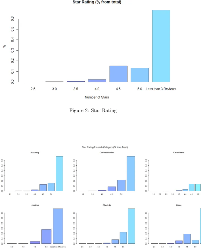
3 Star Rating - Per Categories . . . 22

4 Cancellation Policy . . . 23

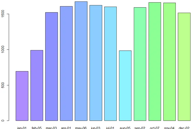
5 Available Listings per date (month-day), where the day is the first friday of the month. . . 24

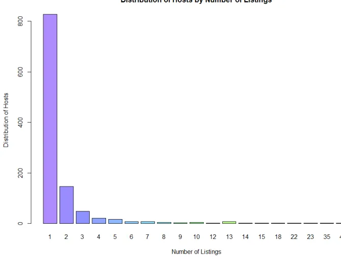
6 Each bar represents the number of hosts with the respective number of listings. . . 25

7 Experience Coefficients . . . 27

8 Seasonality . . . 28

9 Experience Levels . . . 30

10 Summary Statistics per Host Type . . . 31

11 Experience Levels - Professionals x Non-Professionals . . . 32

12 Listing Specific Quality Distribution - Professionals x Non-Professionals . 32 13 ξ Distribution . . . 43

14 Fraction of Rented Listings conditional onξ values (on x-axis) . . . 47

(9)

16 Mean Transaction Price conditional onξ values (on x-axis) . . . 48

17 Mean Transaction Price conditional onξ values (on x-axis) and conditional on rented . . . 49

18 Airbnb initial page . . . 53

19 Airbnb search results page . . . 53

20 Listing page example . . . 54

21 Source code example . . . 54

22 Flexible Cancellation Policy . . . 54

23 Moderate Cancellation Policy . . . 55

24 Strict Cancellation Policy . . . 55

25 Sample B - Frequency of listings per changes . . . 59

26 Sample B - Fraction of listings with price changes per experience . . . 59

27 Sample B - Total available listings per date. . . 60

28 Sample B - % of available listings per date as of available listings in 2015-12-28 . . . 60

(10)

1 Introduction

Peer-to-peer markets are becoming increasingly important and popular as internet access becomes easier and cheaper. In addition, another contributing factor is that people increasingly perceive internet transactions as safe. Basically, these marketplaces enable buyers and sellers1_{to find each other. In these markets, we may see from platforms where}

regular people rent their own goods (e.g.: Getaround and RelayRides for car rentals; StyleLend for apparel and accessory rentals; Airbnb for accomodation) to platforms where people provide their own services (e.g.: TaskRabbit for labor; Lending Club for short-term loans; Care.com for baby-sitting). Along with these new marketplaces, new issues arise. Einav et al. (2015) raise questions about platform design; their impact to the traditional industries and how should be their regulation.

We are interested in studying the learning process in these markets, which is a specially relevant issue concerning them. First, it is important because they are, in principle, characterized by non-professional sellers2 _{who are not used to pricing decisions and with}

no expertise as typical businesses3_{. Furthermore, each of the sellers in those platforms are}

trying to sell her (heterogeneous) products/services in a environment where each seller sets her own prices. Given that, studying how each seller learns about the demand for her product is important both for the platform and for welfare. Depending on how sellers learn, we may see a suboptimal number of transactions in the platform.

It is not hard to think about examples in which the lack or the difficult of learning affects efficiency. In a marketplace for accommodation rentals, hosts without knowledge about their demand may experiment with prices and after frustrating attempts exit the platform. This may be suboptimal because had she known her listing’s demand, she would have rented it, benefiting both herself and the guest. Furthermore, we may have less hosts

1_{The seller does not necessarily has to sell a product, she may rent a product or offer a service; here}

I treat the sellers as the supply side. Alternatively, I treat the buyer as the demand side.

2_{For example, Airbnb, a peer-to-peer accommodation rentals platform, claims that most}

of their hosts are regular people (http://blog.airbnb.com/economic-impact-airbnb/). On the other hand, there are some questioning about this claim (http://tomslee.net/2014/ 05/the-shape-of-airbnbs-business.html).(http://www.huffingtonpost.com/steven-hill/ an-open-letter-to-airbnb_b_8463656.html). Some people claim that professional hosts have high participation on Airbnb’s revenue (http://www.bloomberg.com/news/articles/2016-01-20/ study-professional-landlords-generate-500-million-per-year-on-airbnb),(http://www. ahla.com/uploadedFiles/_Common/pdf/PennState_AirBnbReport_.pdf).

3_{For instance, think about a host that has just joined Airbnb with a listed room against the hotel}

(11)

than the optimal number. A host, when deciding whether to join or not the platform, considers the present value of renting her listing. If she does not know her demand, she incurs in a cost of learning it; differently from the case of perfect information. This cost may offset the benefits from joining the platform. Additionally, we may have less guests than the optimal number due to hosts’ uncertainty about their demand. Suppose that a listing may have two possible valuations (high and low) and hosts know the valuations’ distribution, but not their own values. Thus, they will charge the average value of the listings. A customer willing to rent a low quality accommodation paying the low quality valuation will not transact in the platform as the price charged for it will be higher than its value.

This paper focuses specifically on Airbnb. Airbnb is an online rental marketplace where people can list and book unique accommodations around the world. In this plat-form, potential guests search for a city, dates and number of guests. The search results return a list of listings for the inputs inserted. In this page, potential guests may see for each listing: a listing’s photo, price per night, title, room type, star rating, host’s photo. Entering in a listing’s page, the guest may see additional information. So, given Airbnb’s search mechanism, we may try to track hosts’ behaviour over time. Tracking them over time may give us a hint about how hosts do learn about the value of their listings.

Airbnb is a good setting to study learning for several reasons. First, Airbnb is char-acterized partly by non-professional sellers who are not used to pricing decisions. Since it is a marketplace where people list their own places to rent and each listing has unique features, in principle, they may not know how much potential guests are willing to pay for their listings, i.e., the demand for each listing is uncertain4_{. In addition, rental markets}

are, in themselves, highly uncertain environments, with demand for an accommodation being affected by aggregate shocks as seasonality or even idiosyncratic aggregate ones5

which we do not know how large will be their impacts and/or for how long they will last. Therefore, to properly maximize their profits6_{, hosts have to learn about their listings’}

4_{It may be the case that some hosts already know how is the demand for their listings because they}

used to rent them before joining Airbnb. Furthermore, there may be professional sellers who are used to pricing decisions and know the demand for each listing. However, for those hosts who had never rented their places before, it is difficult to imagine that they know the demand for their listings.

5_{e.g.: Places becoming a must go for a while; Events that may increase/decrease the demand in a}

city/country as Olympic Games or an earthquake

6_{This argument relies on the assumption that hosts tries to maximize their profits with their listings.}

(12)

demand.

In Airbnb, we believe that hosts learn about the demand for their listings mostly through price experimentation. A host learns simply by setting prices (experimenting with prices) and seeing what is the outcome. If she sets a price and does not rent, she may learn that the price is too high and so her listing may be worth less than the listed price. If she rents, she may learn that her listing may be worth at least the set price7_.

Hence, the host learns either if she rents or not. It is important to note that it is costly to experiment - there is a trade-off between experimenting with prices to acquire more information and choosing the optimal price given seller’s current information (exploit current information). To be more specific about what do sellers learn about the demand for a listing, we may think that they may learn their listing-specific quality (consumers’ mean value for their listings) or aggregate demand components (e.g. seasonality).

We develop a dynamic pricing model in which a host has a listing to rent for a spe-cific future date. In each period a potential guest arrives according to a Poisson process. Given that he is present, he decides whether to rent or not the listing, based on both ob-servable characteristics and unobob-servable ones (to the host) (in a discrete-choice model). The unobservable characteristics is decomposed in a listing-specific quality, known to all guests, but unknown to the host; and a idiosyncratic preference shock. The host has uncertainty about her listing-specific quality. She does not observe whether a guest is present; she observes only whether her listing was rented or not. Whenever her listing is not rented, she receives a signal about her listing-specific quality (that quantifies the information she gathered from not renting the listing). The host chooses prices based on her latest information about her listing’s quality to maximize her discounted present value.

As we have specified a discrete-choice model for our demand model, we have to es-timate its parameters. We have specified our demand model as a binary logit model. We estimate it via maximum likelihood to recover listing fixed effects. With the esti-mated fixed effects, we estimate an OLS against observed characteristics to recover the

pay for their places, simply because they don’t care about the money they earn. Even if hosts do not care about money, learning about the demand for their listings may be important for them, because by learning it, they may set prices so that they always have their listings rented and along with it they help the highest number of people. For a discussion about real motivation of hosts to provide their places, seeGutt and Herrmann(2015)

(13)

parameter values. From the distribution of residuals of this second step, we retrieve the parameters of the distribution of the listing-specific quality.

Our data comes from public available data on Airbnb’s website. In the platform’s website, we have information on listings’ prices, characteristics and hosts’ characteristics. We have retrieved them with an automated code in Python. Roughly, the code does what a person would do was he looking for an accommodation in a place, for a specific date and for one guest. First, the code saves each listing page for the specified inputs. Then another code extracts from each saved page the data8_.

We will simulate our dynamic pricing model under three scenarios: a) with learning; b) without learning and c) with full information. The former assumes that the host does not know her listing-specific quality, but knows its distribution. However, she does not learn anything in the selling process. The latter assumes that the host knows its own listing-specific quality. As far as we know, we are one of the first papers to explore learning as an important issue concerning peer-to-peer markets.

The rest of the paper is organized as follows: Section 2 reviews the literature on learning. Section 3describes the institutional details. Section 4introduces the data and some evidence from it. Section5establishes the model. Section6presents the estimation procedure. Section 7presents the results. Section 8concludes the paper.

2 Related Literature

Our paper is related to the learning literature, more specifically to the problem of dynamic pricing under demand uncertainty. In addition, our work is related to the growing literature on peer-to-peer markets.

2.1 Learning

2.1.1 Seller Learning

There is a large amount of theoretical references on learning by experimentation on

8_{One of the drawbacks from our method is that we cannot ensure that we are gathering all the}

(14)

the supply side. One of the first works that brought to economics the problem of pricing under demand uncertainty wasRothschild(1974). He sheds light on the trade-off between experimenting with prices to gain new information about the demand and exploiting the current information, charging the most profitable price given this information. Particu-larly, he finds that if a seller sets prices optimally in a market with unknown demand, then she will eventually end up charging one single price and sticking to it. However, there is no guarantee that the set price will be the one that would be set had the seller known her demand. He models his problem in such way that he can analyze it in a more general framework studied by statisticians and probabilists. From this work on, much economists have studied these kind of problems in which agents try to optimize decisions while improving information simultaneously - known as bandit problems (For a more detailed survey on bandit problems see Bergemann and Valimaki (2006)). Rustichini and Wolisnky (1995) provides an example with demand uncertainty in which demand changes over time in a markovian fashion. In their example, they show that even when the frequency of demand changes is small, there is incomplete learning in the long run. Aghion et al. (1991) consider a more general decision problem in which a decision maker is initially uncertain about the true shape of his payoff function. He learns it over time through observation of the outcomes of his past actions. From this, they characterize conditions under which optimal learning leads to adequate learning9_.

Lazear (1986) tries to explain market phenomenons (as price reduction policies as a function of time on the shelf) through a simple framework which incorporates Bayesian learning. He considers a finite-horizon problem in which a seller has a unique good to sell without knowing buyer’s valuation. She updates her belief about buyer’s valuation based on whether the good was sold or not. He characterized the optimum prices and their behavior over time. Under this general idea, Lazear (1986) considered different hypotheses about consumers, seller and good characteristics to see how would they affect the speed of price changes and the initial price10_.

Chen and Wang (1999) also analyzes a framework in which a seller with a single asset to sell. However, differently from Lazear (1986) who assumes that the valuation is unknown, rather than the distribution, Chen and Wang (1999) consider an infinite time

9_{When, with probability one, the agent acquires enough information to allow him to obtain the true}

maximum payoff

10_{He does not state any proposition or theorem, but rather considers examples to make his point (he}

(15)

framework in which a seller does not know from which distribution the valuation was taken. In the selling process, instead of updating beliefs about the valuation, the seller updates her beliefs about its distribution. Assuming that the valuation may be drawn from two possible distributions, they find a condition - the hazard rate of one distribution is higher than that of the other - under which optimal prices decline over time. Chade and de Serio (2002) consider a similar problem toChen and Wang(1999), but differently from them, the uncertainty relies not only on the distribution of buyers’ valuation, but also on the seller’s reservation price for the good. They characterize the equilibrium and how does the seller’s equilibrium behavior changes when parameters of the problem change. Another related paper to the above works is Mason and Valimaki (2011). In their model, differently from previous works, who assumed that one buyer arrived in each period, buyers arrive randomly according to a Poisson process with an unknown to the seller arrival rate. Buyers’ valuations are drawn from a known distribution. The seller does not observe whether a buyer is present or not, only if a sale has occurred or not. She has a prior over the probability of the arrival rate being high and updates it when no sale occurs. Their main result is that in the case of learning about the arrival rates, the price charged in the presence of learning is greater than the price when there is no learning11 _{for every belief about the arrival rate being high.}

All the papers in the previous paragraphs analyzed the problem of a single seller with a single good to sell, but it is worth noting papers who analyzes sellers with more than one unit to sell. Mirman et al.(1993) consider a two-periods problem in which a monopolist faces an uncertain demand for her good. Her demand curve has an unknown parameter and she maximizes the profits over the two-periods horizon. Firstly, the authors consider a quantity-setting problem and derive sufficient conditions for experimentation for this problem. In addition, they provide conditions under which the monopolist experiments by increasing or decreasing its output (relative to the myopic optimum output). Finally, they compare the quantity-setting and price-setting problems. Keller and Rady (2003) consider a symmetric differentiated-goods duopoly in which firms are uncertain about the degree of differentiation between their goods. The degree of differentiation changes randomly over time according to a Markov process. In each period, the quantities sold

11_{That is, the price charged by the seller when she has a good to sell and does not update her beliefs}

(16)

noisily signal the state of the demand and the informational content of these signals increases with the difference between firms’ prices. They characterize the equilibrium and provide conditions on the parameters that determine whether or not there is price dispersion in equilibrium.

For empirical references on seller’s learning, the most closely related to ours is Huang et al. (2015). They study the market for used cars - products with item-specific hetero-geneity. The authors analyze a structural model to assess how do sellers learn about the demand for their idiosyncratic product in the selling process. Before selling an item, the seller receives a signal about its heterogeneity and whenever the product does not sell, the seller Bayesian updates her beliefs about the item-specific heterogeneity. From their model, they find a decreasing price over time. Through counterfactuals they find that both her initial assessment and learning in the selling process are important to enhance profits.

2.1.2 Buyer Learning

For works related to buyer learning, there is an extensive number of empirical papers on learning on the demand side.

Erdem and Keane (1996) and Ackerberg (2003) analyze how consumers learn about the quality of a product both through consumption and advertising. They consider structural models in which consumers start with a prior on brand quality and update their beliefs about it through consuming and watching advertisements. The key difference between them is the fact thatErdem and Keane(1996) examine only the effect informative advertisements on consumers’ choice, while Ackerberg(2003) considers both informative and persuasive effects12_.

In addition to the marketing literature, it is worth citing the literature on pharma-ceutical demand in which doctors and patients learn about the matching of a drug to the patient. Crawford and Shum (2005) construct a model in which doctors diagnose a patient’s condition and choose a sequence of drugs to minimize his expected disutility from illness. Uncertainty exists both on effectiveness of drugs and the probability that the patient remains ill and drugs affect individuals differently13_{. Patients learn about their}

12_See_Ackerberg₍₂₀₀₁_{) for a detailed discussion about both effects.}

13_{Their main innovation is that they consider two dimensions under which drugs affect individuals:}

(17)

match with each drug through direct prescription experiences. Dickstein (2014) looks at the antidepressant market to measure how drug prices and promotion influence the search process for drug alternatives that best match to patient. He specifies a dynamic discrete choice model allowing both correlated learning between drugs and experimentation14_.

2.2 Peer-to-peer markets

There is a growing body of literature on peer-to-peer markets. Einav et al. (2015) tries to review the literature and shed light on the economic issues surrounding peer-to-peer markets. Among other works, Cullen and Farronato (2014) considers a matching model to study the mechanisms contributing to equilibrate demand and supply when they change using data from TaskRabbit, a domestic task service provider marketplace. Fradkin (2015) also studies matching in online marketplaces using data from Airbnb. He investigates three mechanisms in these markets that cause inefficiences in them: con-sumers cannot consider all possible choices; concon-sumers does not know sellers willingness to transact and transactions happening too early. He proposes a model to study these frictions and possible counterfactuals to them. He finds that potential guests do view only a subset of listings in the market and that there is a relevant fraction of listings remaining vacant for some dates. In addition, hosts reject proposals to transact by potential guests half of the time, causing the latter to leave the market despite having potential match with other hosts. Alleviating these frictions, there would be higher number of matches and higher revenue per potential guest.

Fraiberger and Sundararajan (2015) develop a dynamic model of an economy with a peer-to-peer rental market for durable goods. Consumers are heterogeneous in price sensitivity, utilization rates and preference shocks and decide whether or not to own a car (new or used) and to use a peer-to-peer marketplace. They calibrate their model using data from Getaround - a large peer-to-peer car rental marketplace. They find out that peer-to-peer rental markets improve consumers’ welfare - additionally, they find that they have a large positive effect on lower-income consumers. Horton and Zeckhauser (2016) also consider a model in which consumers decide whether or not purchase a good. Differently from Fraiberger and Sundararajan (2015), there is an homogeneous good.

- impacting a patient’s probability of recovery

(18)

They find that peer-to-peer rental markets improve surplus relative to pre-sharing status quo both in the short and long-run equilibria. Neither Fraiberger and Sundararajan (2015) nor Horton and Zeckhauser (2016) consider the problem of owners setting prices for their good, they take price as given as in a competitive equilibrium.

Additionally, there are some papers analyzing specifically the Airbnb. Gutt and Her-rmann(2015) investigate the motivation of participants on the supply side of the sharing economy using Airbnb data. The paper considers two main reasons for which a host rents his under-utilized inventory: idealism or altruism - because of the ideal of sharing; economic factor - because he wants monetary compensation. They find evidence of eco-nomic factors affecting motivation of hosts15_. _{Edelman and Luca} _{(2015) study the extent}

of racial discrimination against hosts on Airbnb. They find that the gap of rents received by black and non-black hosts persists even controlling for other factors. Fradkin et al. (2015) study Airbnb’s review system. They address the determinants of reviewing be-havior, the information reviews carry with them and changes in the design of reputation system. They note the existence of bias in the reviewing behavior. However, the average rating is compatible with private signals of transaction quality16_{. In addition, from field}

experiments, they find that non-reviewers usually have worse experiences than reviewers. Zervas et al.(2015) investigate the impact of Airbnb on the hotel industry. Hypothesizing that Airbnb’s accommodations worked as a substitute for certain hotel stays, they find that Airbnb’s entry in some markets indeed affected hotels’ performance. In particular, the impact of Airbnb decreased in price tiers segmentation (ie, budget hotels were the most affect and high-end hotels the least). Li et al. (2015) investigate the performance and behavioral differences between professional and non-professional agents on Airbnb. Indeed, they find that professional agents have both higher occupancy rate and daily revenue comparing to non-professional ones. The authors does not find evidence that the better performance of professional agents is due to higher rate of learning.

Another related literature to peer-to-peer markets is the two-sided markets literature.

15_{As identification strategy, the authors consider that if economic factors are the main driver for}

participating in the supply side of the sharing economy, the availability of positive consumer reviews should have a significant effect on prices in the sharing economy. On the other hand, if idealism is the main reason for participation in the sharing economy, this availability should not affect prices, but rather affect the utility of hosts in non-monetary ways. They find that rating visibility in fact causes hosts to increase their prices.

16_{They explore a feature from Airbnb’s review system in which guests are asked if they recommend}

(19)

These markets are characterized by two distinct groups of agents, each one interacting with the other. Their interaction is intermediated by a platform, who seeks to maximize its profits choosing the best choice of fees between both sides. Airbnb has characteristics of a two-sided market. It allows potential hosts and guests, who benefits from transacting to the other side, to meet each other and charges each side according to its objective. Li et al. (2015) highlight that one of the crucial differences between sharing economies and traditional two-sided markets is the fact that the supply side in the sharing economy is characterized both by professional and non-professional players. Besides investigating differences in performance and behavior between them, they consider a two-sided market model to incorporate this difference in one side of the platform to derive the optimum prices charged by the platform and by the social planner.

3 Institutional Details

Airbnb is an online marketplace for people to list and book unique accommodations around the world. The platform was founded in 2008 and it claims to have over 2 million listings in over 34 thousand cities and 190 countries.

Although there were already marketplaces for people to list their accommodations, these marketplaces focused on entire homes/apartments rentals and they worked more as an advertising platform, without participating in the transaction. One of the main innovations of Airbnb was the possibility to list not only entire homes/apartments, but also parts of an apartment (private room/ shared room). Furthermore, along with a strong system of trust and reputation to enhance the security of transactions, it established a payment mechanism in which the payment had to go through the platform. In a transaction, Airbnb holds the guest‘s payment and releases it to the host only 24 hours after the guest checks in. The security deposit is also intermediated by Airbnb.

(20)

sees additional photos, amenities, space, prices, description, house rules, reviews, star ratings and additional host information. Next, the guest chooses which accommodation to book and contacts the host inquiring about room details and availability. A host may answer that room is unavailable, that it is available or by asking a follow up question. He may also not respond at all. After both parties agree, the guest can finally book it. If host accepts, the money is charged and held by the platform until 24 hours after the guest’s check in. After the booking, further communication is held to exchange keys and coordinate the details of the trip. Cancellation may apply with pre-established penalty rate. After check out, during a period, both parties are asked to review each other (See Fradkin et al. (2015) for further details about the review system).

For the host, Airbnb provides a service of management of pricing and property calen-dars and recently it launched a pricing tool to help hosts to price their listings. The host sees a calendar with price per night for each date. In addition, for each date she can mark his listing as available or unavailable. If a booking occurs, her calendar is automatically blocked off for the booking dates. So for those booked and blocked dates, the property cannot be booked and will not show up in search for the blocked off dates. The pricing tool is based on a daily updated machine learning that shows how likely a guest is to book a specific listing, on specific dates at a range of different prices. Given a listing, for each date this tool gives a price tip to her listing and shows through a line that changes its color, how likely she is to rent her listing for each price she sets.

Concerning the platform’s revenue, Airbnb makes money charging from the guests a 6% to 12% service fee over the reservation subtotal. The higher is this subtotal, the lower the percentage guests pay. Additionally, Airbnb charges a 3% host service fee for payment process over the reservation subtotal. (e.g.: Consider a $200/per night for 7 nights and $150 Cleaning fee reservation - the reservation subtotal is $1550; Airbnb will charge 6% to 12% of $1550 from the guest and 3% of $1550 from the host).

(21)

number of websites specialized in price management and price consultancy for hosts 17_.

4 Data

In this section, we describe how the dataset was constructed and some summary statistics from it.

4.1 Data Extraction

The data was scrapped from Airbnb’s website. Our code was made in Python. The code does what a potential guest may do to find a listing to book.

First, you set in the code the check-in and check-out dates (you may insert a vector of dates), city and state that you want to retrieve the data (The code takes the number of guests as one).

Additionally, you set the number of intervals you want the price vector to have (e.g.: You want 10 intervals; the price goes from 40 to 4000; so the price vector will be [40,436,832,1228,1624,2020,2416,2812,3208,3604,4000]). The code takes this informa-tion and insert in the Airbnb browser.

Next, in the search results page 18_{, the code iterates over dates, room types,}

neigh-borhoods and price ranges in price vector to retrieve the HTMLs from each of the listings and save them in the computer.

Then, another code opens each of these listing’s HTML pages and retrieve the infor-mation from each page.

In summary, first the code enters the input information (place, dates, number of guests) in the airbnb initial page (Figure 18 in appendix). Next, in the search results page, the code filters the listings by prices and room type, iterating over them.(Figure19

in appendix). In each of the filtered search results page, the code enters in each listing page and save its HTML (Figure20in appendix). Each HTML contains the source code from the listing page, which, in turn, contains all the information we want (Figure 21in appendix). Then, another code gather all information from those source codes and save

17_{For examples} _{https://www.pricelabs.co/}_; _{https://www.everbooked.com/}_; _https://www.

pricemethod.com/.

18_{It is important to note that the search results page only displays the available listings, i.e., those}

(22)

them in a CSV file.

In our exercise, we work with a scraped dataset for Ipanema, Rio de Janeiro, RJ. The sample is a cross section that was scraped for the first week of each month of 2016 starting from Friday and for no date inserted 19_{. The no date data stands for all listings}

in Ipanema, Rio de Janeiro, RJ, independently if the listing is available or not. The code ran just once, but took 9 days to finish. This sample was extracted on 11/24/2015 to 12/03/2015.20

4.2 Data Description

In this section, we will describe the dataset we gathered from the website. It is important to highlight that two shortcomings of our dataset are: 1) we only have price data on available listings for a date; 2) we cannot ensure that non-available listings are rented because non-availability may come from hosts not willing to rent. Furthermore, since we only see available listings, all analysis have to be carried with caution due to the possibility of sample selection.

In a listing page, we see several sections divided in: space, amenities, price, reviews, about the host and other sections with descriptions of the listing and house rule. In addition, there is a price table.

The space section describes the general structure of the listing. This section shows how many people the listing accommodates, the number of bathrooms, bedrooms and beds. In addition, it shows bed type, check-in and check-out hours, the property type (Ipanema has apartments, lofts and houses; but more generally we may see castles, chalets, huts, boats and other property types) and room type (Entire home/apt, private room or shared room). Shared rooms as the name suggest stands for rooms where the guest shares the bedroom and the entire space with other person(s). If the guest chooses a private room, he will have a bedroom for himself, but will share some spaces with others. When the

19_{(01/01/2016 to 01/08/2016; 02/05/2016 to 02/12/2016; 03/04/2016 to 03/11/2016; 04/01/2016}

to 04/08/2016; 05/06/2016 to 05/13/2016; 06/03/2016 to 07/01/2016; 08/05/2016 to 08/12/2016; 09/02/2016 to 09/09/2016; 10/07/2016 to 10/14/2016; 11/04/2016 to 11/11/2016; 12/02/2016 to 12/09/2016)

20_{In the appendix, we display another scraped sample. This sample is a panel data that was scraped}

(23)

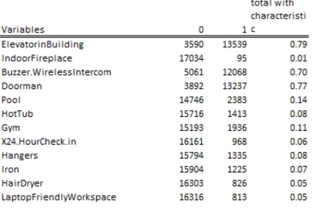
Table 1: Amenities

guest chooses an entire home/apt, he will have a whole space for himself.

The amenities section shows a list of amenities that the host may offer to the guest. In the table 1, we show the list of amenities and their proportion in the sample. In our data, each of the variables is represented by an indicator, which assumes value 1 if the listing has the amenity and 0, otherwise.

(24)

control of the host?), for communication ( how responsive and accessible was the host before and during your stay?), for location ( how appealing is the neighborhood (safety, convenience, desirability?) and for value (how would you rate the value of the listing?). All these ratings are anonymous star rating 1 to 5 stars. The results of all reviewers are averaged out and shown on listing’s page. It is important to mention that Airbnb displays star ratings only after 3 reviews are submitted. Furthermore, this section displays what guests have said about the listing. We do not retrieve the reviews’ contents.

There is a section that displays information about the host. This part displays a host photo, information about where she came from, when she joined Airbnb, if she has verified ID (if the host has completed online and offline ID verification) and total number of reviews (including reviews from other listings from her). We retrieved only the infor-mation about when she joined the platform21_{. We have defined variables corresponding}

to months of experience as the difference between a reference date and the date that the host joined. The reference date is November 2015, because we have retrieved the data in November 2015.

After setting check-in, check-out and number of guests in the listing page, the price table updates the price per night and other fees. This table displays the price per night, price per night times length of stay, cleaning fee, service fees and the total amount after fees.

Furthermore, there are more information displayed in a listing page as a description section, a house rules section and a minimum stay section. We do not retrieve them because texts are difficult to be quantitatively interpret. The minimum stay section displays the minimum number of nights a guest can rent set by the host. The host can set different minimum stays for different dates, so this information is not so reliable. In addition, there are photos of the listing.

The following table (Table 2) displays some summary statistics about some variables described above for the sample. Note that in our sample most of the observations have a few number of reviews (75% of the sample have less than 5 reviews).

The data set is a cross section with 17129 observations22_{. Each observation is defined}

21_{The airbnb website used to display Response rate and Response time - variables that measured}

how often and how fast hosts used to answer questions received. Since mid-December 2015, the website stopped to display them. In 2016, they started again to display the information.

22_{We have dropped listings whose host had more than 57 months of experience. In addition, this}

(25)

by a (listing ID, date)-pair, in which listing ID is a unique number that identifies a listing and date is the check-in date for the listing ID23_{. We have that the sample is in}

a long format. For each observation, we have listing’s prices, characteristics and host’s characteristics.

Table 2: Summary Statistics

Figure 1: Room Type

23_{So, if a listing was available all specified dates, we would have 13 observations corresponding to this}

(26)

Figure 2: Star Rating

(27)

Figure 4: Cancellation Policy

(28)

(29)

Figure 6: Each bar represents the number of hosts with the respective number of listings.

(30)

non-negligible number of hosts with more than one listing. These figures are important, because depending on how we define a professional seller24_{, we see that they account for}

a non-negligible fraction of the hosts in the platform. Also, this shows that in fact the platform is characterized by non-professional sellers25 26_.

4.3 Preliminary Findings

In this section, we focus on patterns we see in the Airbnb. It shows some reduced form evidence consistent with learning. In particular, we show that: 1) Experience of a host affects her pricing behaviour and 2) There are constant demand and supply shocks that reinforce the importance of learning.

4.3.1 Experience

For this part, we considered the following regression:

Pjm=Xjβ+

12 X

i=1 Di+

19 X

k=1

expdummyk+εjm (1)

wherePjmis the price per night of listing j for date m;Xj is a vector of controls for listing

j(number of reviews, dummies for each level of overall satisfaction, dummies for cancel-lation policy, dummy for internet, air conditioning, free parking on premises, doorman, TV, breakfast, Gym, Pool, Kitchen; Security Deposit and room type). Di fori= 1, ...,12

represents a dummy for each date of rental (one for each month). We have created 19 experience dummies (expdummyj), one for each interval of three months. For instance,

a expdummy3 = 1 means that the host has from 6 to 9 months of experience.

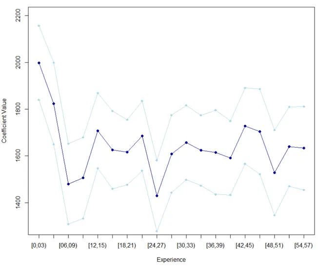
The figure 7 plots the coefficient estimates for each experience label dummy and its respective 95% confidence interval. From the figure, it seems that less experienced hosts (Those with less than 6 months of platform) charge higher prices comparing to more experienced ones. This figure is in line with a learning explanation in which those

24_{Li et al.}₍₂₀₁₅_{) define professional hosts as those who offer two or more unique units.} _Schneiderman

(2014) define professional hosts as those who offer three or more unique units.

25_{Independently on how we define them.}

26_Schneiderman₍₂₀₁₄_{) note in the data provided by Airbnb for New York city that in his sample only}

(31)

hosts who have less experience join the platform experimenting with higher prices to gain information, then as time passes (renting or not) they adjust their prices downwardly until a certain point, after which they start to exploit their information.

(32)

4.3.2 Demand/Supply Dynamics

This subsection displays some figures about the constantly changing nature of the environment that hosts face in the platform. We try to show that both demand and supply are affected by shocks that, in principle, a host may not know how they affect their listings. Hence, she has to learn about them to optimally price her listing.

Pjm =Xjβ+

12 X

i=1

Di+εjm (2)

Figure 8: Seasonality

(33)

on prices. In August 2016 Rio de Janeiro is hosting the Olympic Games, so this will be a high demand period27_{. Given that, hosts also increase their prices for the period to take}

advantage of the high demand. Since the Olympic Games are not an event that takes place every year in Rio, we cannot account this effect as a seasonal effect. Even so, it is important to document this effect as hosts, to fully take advantage of the high demand and to not leave money on the table, have to understand the extent to which this event will affect the price for their accommodations.

Although the above story may seem plausible, we cannot guarantee that these effects are caused by those events. Recalling figure5, we see that those months with pronounced effects on prices are exactly those months with less available listings. Another story that may explain these estimates is the existence of sample bias. It may be the case that on those dates with less available listings, the remaining listings are exactly those with very high prices. Hence, the estimates we are retrieving from these months are not reflecting the seasonality/event effects, but the fact that we are not using a representative sample of the listings.

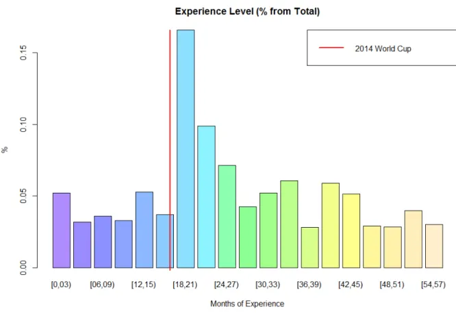
From the figure 9, we have the number of observations with a given experience level. There is a high fraction of observations 18 to 27 months of experience (26%). This number may reflect the world cup and hosts joining the platform to rent their places for the event (World Cup in Brazil happened 17 months before the scrape date. Hence this effect may reflect hosts who joined the platform to rent for the event). This figure shows evidence that the supply responds to demands shocks. As a consequence, the host has to learn how this supply response will affect her residual demand.

27_The _games’ _local _organizing _committee _is _counting _on _the _Airbnb’s

(34)

Figure 9: Experience Levels

4.3.3 Professionals x Non-Professionals

In this subsection, we look to the difference between professional and non-professional sellers. We define professional sellers as hosts with more than one listing and non-professional ones as those with only one listing28_.

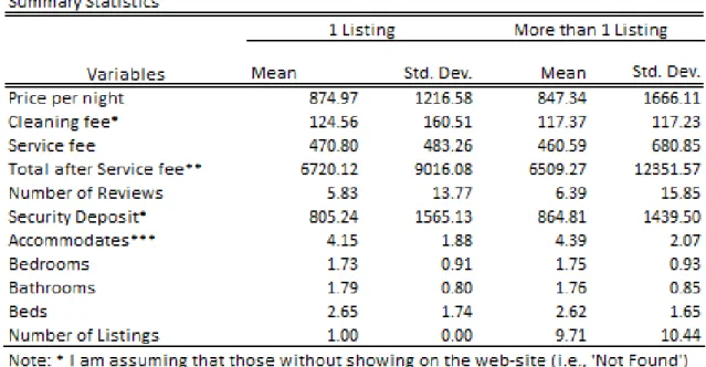
Figure 10 displays some summary statistics by type of seller. From the first row we see that observations whose host has a single listing have higher mean prices per night comparing to those whose host has more than 1 listing. Furthermore, their prices are less dispersed than the latter. In addition, hosts with one listing charge on average higher cleaning fees. Looking to the space, observations whose host has only one listing are similar to those whose host has more than 1 listing.

Figure11depicts the experience coefficients from regression (1) for observations whose host has only one listing; whose host has more than one listing and for all sample. The green line displays the same figure as figure 7. We can see a clear difference between mean prices for hosts with less than 18 months of experience for professional and

non-28_{This is an ad hoc definition;} _Schneiderman ₍₂₀₁₄_{) considers as professional sellers as those with}

(35)

Figure 10: Summary Statistics per Host Type

professional sellers. Specifically, professional hosts with less than 18 months of experience charge on average higher prices than non-professional ones.

(36)

Figure 11: Experience Levels - Professionals x Non-Professionals

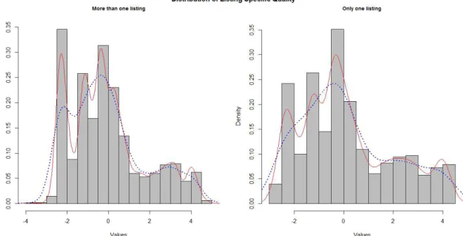
Figure 12: Listing Specific Quality Distribution - Professionals x Non-Professionals

5 Model

(37)

Consider a setting with J hosts, each one with a single listing who sets a sequence of take-it-or-leave-it prices over time for a listing j to rent for T+1 periods ahead. Time is discrete and is denoted by t=0,1,...T. The listing quality is known by consumers, but not known by the host. At the start of each period, the host sets the price for that period. If the potential guest is willing to rent at that price, the host rents her listing and the problem ends. The host discounts the future at rate δ.

Potential guests arrive randomly according to a Poisson process. With an arrival rate λ, in any given interval (t, t+ 1], there is a probability of (1₋e−λ_{) of at least one}

potential guest be present. We will assume that λ is known to everyone. Furthermore, we will assume that from all potential guests that arrived, only one will be assigned to decide whether to rent or not.

Listing’s quality is drawn from a normal distribution that affects directly the renter’s utility, entering additively in his utility function. The host does not observe whether a potential guest is present or not. She only observes if the listing was rented or not. Hence, the probability of rental in any given period, given a listing’s quality, is given by the probability of at least one potential guest to be present times the probability of the listing to be rented, conditional on the guest being present. The latter probability depends on the host’s belief about her listing’s quality. The host initially believes that her listing-specific quality follows a normal distribution drawn from the population distribution of quality.

The state variable of the problem is the host’s belief about the parameters of the distribution of her listing quality and time to the event. The only event that is relevant for updating her beliefs is when no rental occurs in a period (because when the listing is rented, the problem ends). To quantify the information she receives when she does not rent, whenever she does not rent, she receives a signal centralized in her true listing quality with a white noise. She updates her prior in a Bayesian fashion.

5.1 Arrival Rate

Potential guests arrive randomly according to a Poisson process. This process de-scribes the number of arrivals that occurs in a given period. Hence, with an arrival rate

(38)

Prob(N(a, b] =n) = (λ(b−a))

n

n! e

−λ(b−a) ₍₃₎

whereN(a, b] is the number of potential guests arriving in (a, b]. In particular, in (t, t+ 1] we have:

Prob(N(t, t+ 1] =n) = (λ)

n

n! e

−λ ₍₄₎

That said, the probability that at least one potential guest arrives to listing j in (t, t+ 1] is:

Prob(N(t, t+ 1]≥1) = 1−Prob(N(t, t+ 1] = 0) = (1−e−λ) (5) In principle, λ may be unknown. We will assume that it is known.

Given that at least one potential guest is present, assume that only one of them in fact decides whether or not to rent the listing j at t. We may think that in (t, t+ 1] the host receives a number of inquires and decides not to reject only one of the them, leaving only one potential guest to decide whether or not to rent the listing. If potential guests are present, the assigned one to take the decision chooses whether to rent or not. After that, he exits the market. The decision of each potential guest is independent from other guests’ decisions.

5.2 Renter’s Problem

LetUjt be the utility from the renter for the listing j at time t, given that he is present:

Ujt =Vjt + ˜ǫjt (6)

Vjt is the part of the utility observed by the the host, but ˜ǫjt are factors that affect the

guest’s utility, but are not observed by the her. Vjt is specified as it follows:

Vjt =Xjβ+αpjt (7)

and ˜ǫjt as:

˜

ǫjt =ξj +εjt (8)

(39)

listing-specific time-invariant quality known to guests, but not to the host; εjt is the preference

shock for j at t29_. _β _and _α _{are fixed coefficients that do not vary across listings.}

So (6) may be written as:

Ujt =Xjβ+αpjt+ξj +εjt (9)

Let U0t be the value that the potential guest receives if he does not rent any listing,

given that he is present:

U0t=ε0t (10)

Assume that εjt and ε0t are iid extreme values for every period t and across j. Also,

assume that they are independent fromξj.

Define

It=✶{Ujt > U0t} (11)

It is an indicator of renter t choosing to rent listing j. Guest t rents j if and only if this

choice gives him the highest utility.

Conditional on a potential guest being present, given (Xj, pjt, ξj) and recalling that

εjt andε0tare iid extreme values, we have that the probability that the present potential

guest that arrives at t chooses j is:

Eεt[It|Xj, pjt, ξj,Buyer is Present] =Pr(Ujt > U0t|Xj, pjt, ξj,Buyer is Present)

= e

Xβ+αpjt+ξj

1 +eXβ+αpjt+ξj = D(Xj, pjt, ξj) (12)

The expression above gives us the probability of renting the listing at t, given time-invariant observable characteristics, price at t, listing-specific quality and that a guest is present. Since ξj is unknown to the host, she cannot condition her decision on ξj. Thus,

the demand the host faces is the expectation of D(Xj, pjt, ξj) over the possible values of

ξj:

29_{Note that from our assumption that given that a potential guest is present, only one is fact is a}

(40)

Eξ[It|Xj, pt,Buyer is Present] =Eξ n

Eεt[It|Xj, pt, ξj]

Xj, pt,Buyer is Present] o

=Pr(Ujt > U0t|Xj, pt,Buyer is Present)

=

Z

D(Xj, pjt, ξj)g(ξj|θ)dξj (13)

wheref(ξj|θ) is the distribution ofξj with distributional parameters θ. (13) gives us the

expected demand for listing j at t given that a guest is present.

5.3 Host’s Problem

In this section, we describe the dynamic pricing models we will be working with. We consider three models: with learning, without learning and with full information. The difference between them is the hypothesis about the knowledge about ξ. A common feature of the three settings is the finite time horizon. Furthermore, we assume that the continuation value after that last decision period T is zero.

5.3.1 Learning Process

Before specifying the host’s problem, we have to detail her learning process. We will adopt a similar to Huang et al. (2015) learning process. The host is uncertain about

ξj, which is her listing-specific quality. Since ξj is unknown, she treats it as a random

variable. Being more specific, the host has a initial distribution of belief about the value ofξj upon which she makes her first pricing decision. She can learn aboutξj through the

rental process, updating her beliefs when no rental occurs in the period (if she rents, the problem ends).

Since the host does not know her true listing-specific quality ξj, she has a prior belief

about the distribution of this value. We will assume that she believes thatξj ∼ N(µ1, σ12).

Thus, before setting the price for the first guest, she believes that ξj is drawn from a

normal distribution with meanµ1 and varianceσ21. We assume thatµ1 =µand σ12 =σ2,

the population’s parameters.

(41)

and εjt. She updates her belief about ξj using Bayes’ rule whenever she receives a new

signal.

To fix ideas, the story is as it follows: a host joined Airbnb with a listing without knowing how much guests value her listing, controlling for observables. She believes that her listing-specific quality ξj is drawn from a normal distribution with ξj ∼ N(µ1, σ12).

After engaging in the rental process, if she does not rent her listing at t=1, she receives a signal yj1 and updates her belief about ξj and the game continues. Otherwise, she rents

her listing and the game ends. Let yt ₌ _{_y

1, ..., yt} be the history of signals up to the tth arrival of potential guest

(after receiving t ’rejections’). µt+1 is mean of the host’s belief about ξj after observing

t (the history yt_{) signals and} _σ

t+1 its variance.

5.3.2 Problem with Learning

The host does not observe whether a guest is present, she only observes if her listing was rented or not. Thus, in a host’s view, the probability that a rental occurs in any given period (t, t+ 1], given arrival rate λ is:

Prob(Rental occurs in t) = (1₋e−λ₎h Z

D(Xj, pjt, ξj)g(ξj|θ)dξj i

(14)

The host updates her belief when she does not rent the listing in a Bayesian fashion. From appendix9.4, we have that the host updates her belief about the parameters of the distribution g(ξj|θ) in the following way:

µt+1 = σ2

ǫµt+σt2yjt

σ2

ǫ +σt2

=µt+qt(yt−µt) (15)

σ_t2₊₁ = σ

2

tσ2ε

σ2

t +σε2

(42)

whereqt= σ 2

t σ2

t+σǫ2 may be interpreted as the speed or degree of learning

30_{. Let}_V

t(.) be the

value function of the seller in state θt = (µt, σ2t) at t, we have that the host maximizes

the following equation:

Vt(θt) = max pjt

pjt(1−e

−λ₎h Z

D(Xj, pjt, ξj)g(ξj|θt)dξj i

+

δn1₋(1₋e−λ₎h Z

D(Xj, pjt, ξj)g(ξj|θt)dξj io

Eµjt+1

Vt+1(θt+1)

(17)

Fort= 1,2, ..., T−1, whereθtevolves according (15) and (16); andyjt ∼ N(ξj, σt2+σǫ2).

The first term on the right side is the current expected profit from setting pricepjt and the

second is the discounted expected value from setting pjt. This second term is composed

by a discount factor, the probability of no rent occurring at t and the expectation of the value function at t+1 . The expectation is taken overµjt+131, which is the possible values

for the mean of the distribution of ξj. Note that we do not need to integrate over σt2+1,

as this variable evolves deterministically. In addition, VT(θT) is given by:

VT(θT) = max pjT

pjT(1−e

−λ₎h Z

D(Xj, pjT, ξj)g(ξj|θT)dξj i

(18)

Since the problem is a finite time horizon problem, we can solve it by backward induction. First, given θT, we solve (18). Then, with VT(θT), we input it on (17) evaluated at

t = T −1 and solve it. Then, we repeat this procedure for t = T −2, T −3, ...,1 (See appendix 9.5).

30_{Writing (}₁₆_{) in terms of the initial prior, we have that} _σ2

t = σ21σ

2 ǫ

(t−1)σ2 1+σ

2

ǫ. Then, we can write qt as qt =

σ2 1

tσ2 1+σ

2

ǫ. From (15), we have that as qt goes to zero, signals have less weight in the prior updating and consequently become less important in the host’s posterior. In the extreme case ofqt= 0,

we are in the case of no learning as µt+1 = µt, ∀t = 1,2, ...n. Assuming σ21 > 0, if σǫ2 is very

high, signals are very dispersed, implying in a smaller speed of learning, ceteris paribus. As σǫ2 →

∞ ⇒ qt → 0, signals become so dispersed that hosts do not learn anything. Note that, as time

passes by, signals become naturally less important to host’s prior update. Alternatively, as qt goes

to one, signals have more weight in the prior updating and consequently become more important in the host’s posterior. Assuming σ21 > 0, if σǫ2 is very low, signals tend to be very close to the true

parameter ξ, implying in a higher speed of learning. In the extreme case of qt = 1 (σǫ2 = 0), we have

that the host learns completely after the first signal µ2 = y1 = ξ. Note that we can write µt+1 as

µt+1=µ1

t

Q

k=1

(1₋qk) + t−1

P

m=1

t

Q

k=m

(1₋qk+1)qmξ+qtξ+ t−1

P

m=1

t

Q

k=m

(1₋qk+1)qmǫm+qtǫt.

31_{There is a map between}_y

(43)

5.3.3 No Learning

In this subsection, we describe the host’s problem assuming that she knows the popula-tion’s quality distribution, but she does not update her belief about her listing’s quality. Since she faces the same demand function every period, we have that her problem is:

Vt(θ1) = max

pjt

pjt(1−e

−λ₎h Z

D(Xj, pjt, ξj)g(ξj|θ1)dξj i

+

δn1₋(1₋e−λ₎h Z

D(Xj, pjt, ξj)g(ξj|θ1)dξj io

Vt+1(θ1) (19)

VT(θ1) = max

pjT

pjT(1−e

−λ₎h Z

D(Xj, pjT, ξj)g(ξj|θ1)dξj i

(20)

where θ1 is her initial belief about the parameters of the listing’s quality distribution.

Note that the difference from these equations to (17) and (18) is the fact that in the no learning case the host begins with θ1 and does not change her prior.

5.3.4 Full Information

In this subsection, we assume that the host knows exactly the value of her listing specific quality ξj. Since she faces the same problem every period, her problem is:

Vt(ξj) = max pjt

pjt(1−e

−λ

)hD(Xj, pjt, ξj) i

+

δn1₋(1₋e−λ₎h_D(_X

j, pjt, ξj) io

Vt+1(θ1) (21)

VT(ξj) = max pjT

pjT(1−e

−λ₎h_D(_X

j, pjT, ξj) i

(22)

where ξj is known to the host.

(44)

6.1 Demand Estimation

In this section, we describe our estimation methods. We will estimate the parameters of our demand model using a logit model estimation method. From the model’s residuals, we retrieve the empirical distribution of listing-specific quality and simulate the dynamic pricing model.

To estimate our demand model, we assume that the unavailability of a listing for a date means that the listing was rented for that date, acknowledging that it may contain measurement errors. Since for those unavailable listings for a date we cannot see their prices, we use hedonic prices to fill missing prices. With the sample, we run the following regression:

pjt =F Et+F Ej +errorjt (23)

whereF Etstands for date fixed effects (jan-16,feb-16,...,dec-16) andF Ej stands for listing

fixed effect. With the estimated coefficients, we predict the prices for the unavailable listings for each date according to predicted counterpart of (23). Then we construct a new dataset, containing the observations from the sample and the unavailable ones32_.

From the data we have to recover 2 sets of parameters: the observed characteristics’ coefficients (including the price coefficient) and the parameters of the distribution of listing-specific quality. Differently from the model specified in section 5, in our main specification, we estimate a logit demand considering listing fixed effects, that captures both the observable characteristics and what we have called listing-specific quality. Next, we regress this fixed effects on the observable characteristics. The distribution of the residuals of this second regression determines the parameters of quality distribution. We estimate the demand using maximum likelihood. Note that the probability of happening the outcome (rental or not) that was actually observed for listing j for period t is given by33_:

eF Ej+αpjt

1 +eF Ej+αpjt

djt 1

1 +eF Ej+αpjt

1−djt

(24)

32_{The was treated so as to contain 17032 observations. Completing this sample with those unavailable}

ones, we finished with 23640 observations. Among 6608 predicted missing prices, 109 were negative. Those 109 predicted missing prices corresponded to 23 listings at total. We have dropped all observations associated with them giving a total of 23x12 = 276. So we finished with a estimation sample with 23364 observations.

33_{Although not specified, we have controlled for time fixed effects. In addition, we have excluded}

(45)

wheredjt = 1 if the listing was rented and zero otherwise. This is simply the probability

of the observed outcome for listing j and time t.

Recalling that the decision of each individual who arrives to j for period t is indepen-dent from other decision makers, the probability of observing the outcome for all listings and periods that was actually observed (the likelihood function) is:

L(α, β) =

12 Y t=1 J Y j=1

eF Ej+αpjt

1 +eF Ej+αpjt

djt 1

1 +eF Ej+αpjt

1−djt

(25)

The log-likelihood function is then:

LL(α, β) =

12 X t=1 J X j=1 djtln

eF Ej+αpjt

1 +eF Ej+αpjt

+ (1−djt)ln

1

1 +eF Ej+αpjt

(26)

Hence, our objective function is to find the parameters (α, β) to maximize (26). Actually, we have dealt with this using a function in R (glm()) that approaches the logit model as a generalized linear model and finds the maximum likelihood estimators via iteratively reweighted least squares (IWLS/IRLS).

After estimating the demand model, we recover the listings’ fixed effects ˆF Ej and

run an OLS against listings’ observed characteristics. Note that the error of the model encompasses the listing-specific quality.

ˆ

F Ej =Xjβ+υj (27)

With ˆυj, we take its empirical distribution and extract its parameters to describe the

distribution of listing-specific quality.

6.2 Dynamic Pricing Simulation

For our dynamic pricing model simulations, we have to parametrize not only demand parameters, but also parameters from the dynamic pricing model in itself. At total, we have to determine seven parameters (µ, σ2_{, σ}2

ǫ, α, β, λ, δ). µand σ2 as already mentioned

(46)

take its mean. λ will be set exogenously to 2. This leads the probability of at least one guest to be present in each period to be 86.47%. δ is also set exogenously to 0.99. Note that, in principle, we should have usedαas estimated from the demand model. However, as the results will show, this coefficient, although significant is very close to zero. Since this coefficient was generating a demand almost not sensitive to price and hence a corner solution34_{, we have adopted another approach to determine}_α_{. More specifically, we have}

chosen αand σ2ǫ to closely match the mean price, conditional on the listing being rented,

of our sample (given the parameter values from above).

7 Results

7.1 Demand

Table 5 shows the demand estimation under different specifications and 6 shows our main specification. In the specifications in table 5, we have used the whole sample. For our main specification, we have used a sample excluding listings with all dates available, i.e., without any rented date. Note that the price coefficients, although significant, were very close to zero. We do not believe that demand do not respond to prices35_{. We believe}

that the main issue driving this effect is a measurement error on prices. Recall that we have input the missing prices with an hedonic pricing regression. What may be happening to our imputation is that we are attributing to rented observations, prices that are higher than the real transaction ones36_{. Nevertheless, note that we should not expect a very}

high coefficient estimate of the price coefficients. As it will be seen, we could fit the mean price conditional on rented listings with a price coefficient value of -0.00405.

The distribution of listing-specific quality derived from (27) is depicted in figure 13. Note that this empirical distribution is clearly skewed to the right. However, we will take it as if it were a normal distribution, described by the mean and the variance of

34_p

t→ ∞; computationally this leads to a price in the maximum point in the grid

35_{Note that in our main specification instruments are not very useful as they are used to control for}

non-observable variables correlated with an independent variable. Since we have used listing fixed effects, we have controlled for all listing’s unobserved heterogeneity that may be correlated to the independent variable.

36_{e.g.: Think about a listing with January to September being available, but with October to}

(47)

the empirical distribution. The mean is 0 and the variance 3.402. In summary, the parameters are described by table 4.

Table 4: Parameters

Parameter Value Method Description

µ 0 Mean of the distribution of residuals of (27) Mean of the distribution ofξ

σ2 _3.405 _{Variance of the distribution of residuals of (}₂₇₎ _{Variance of the distribution of}_ξ

Xβ 2.19 Mean of the fitted values from (27) Mean impact of observed characteristics

λ 2 Set Exogenously Parameter of Poisson Distribution

δ 0.99 Set Exogenously Discount Factor

σ2

ǫ 50 Set along withσǫ2; Target: E(pjt|rented) = 968. Variance of signal shocks

α -0.00405 Set along withσ2

ǫ Target: E(pjt|rented) = 968. Price Coefficient

T 12 Set Exogenously Number of Periods

(48)

Table 5: Demand Estimation

Dependent variable:

rented

(1) (2) (3) (4) (5)

Flexible Cancellation 0.335∗∗∗

(0.093)

Moderate Cancellation 0.413∗∗∗

0.788∗∗∗ (0.062) (0.107)

Strict Cancellation 0.093∗∗

0.423∗∗∗ (0.038) (0.094)

Number of Bedrooms −0.048∗∗∗

−0.003 (0.018) (0.019)

Number of Reviews −0.002∗

−0.002∗ (0.001) (0.001)

Visible Stars (1 if visible) −1.419∗∗∗

−1.734∗∗∗ (0.326) (0.350)

Visible Stars*Number of Stars 0.342∗∗∗

0.410∗∗∗ (0.069) (0.075)

Private Room Dummy −0.333∗∗∗

−0.407∗∗∗ (0.049) (0.053)

Shared Room Dummy 0.696∗∗∗

0.762∗∗∗ (0.161) (0.172)

Internet 0.366∗∗∗

0.400∗∗∗ (0.074) (0.079)

Air Conditioning −0.106∗

−0.112∗ (0.058) (0.063)

Price with cleaning fee 0.00004∗∗∗

−0.00004∗∗∗

−0.0001∗

0.0001∗∗∗

−0.00004∗∗∗ (0.00001) (0.00001) (0.00005) (0.00001) (0.00001)

Constant −1.005∗∗∗

−1.286∗∗∗

(0.017) (0.076)

datenum No Yes Yes No Yes

ListingID No No Yes No No

Observations 23,364 23,364 23,364 23,364 23,364 Log Likelihood −13,746.780 −12,262.770 −6,821.538 −13,640.730 −12,147.130 Akaike Inf. Crit. 27,497.560 24,551.530 17,561.080 27,305.450 24,340.260

Note: ∗

p<0.1;∗∗